


Is Geography Destiny?
The jury is in—three decades of increasingly-restrictive land use regulations are driving up the cost of housing. Policy makers and economists agree that regulatory reform is essential to restoring affordability in our high-growth cities and metropolitan areas.1 These regulations limit increases in the supply of housing and thus boost house prices and rents. The National Association of Home Builders estimates that government regulations now account for about a quarter of the final price of a new single-family home built for sale.

Zoning and other local land use regulations have increased over the last three decades, particularly in high-growth cities and metropolitan areas.1 A 2016 study by Paul Emrath of the National Association of Home Builders found that government regulations account for 24.3 percent of the final price of a new single-family home built for sale. These regulations limit increases in the supply of housing and thus boost house prices and rents.
These types of regulations impose significant social costs. High housing costs create barriers that prevent workers from moving to high-growth, high-wage cities. These barriers strand many workers in low-productivity industries. Hsieh and Moretti estimate these barriers lowered aggregate U.S. growth by more than 50 percent from 1964 to 2009.2
But is regulation the only, or even the principal, culprit for high housing costs and its impacts? Consider the following transaction in West Seattle, historically an affordable enclave in the now-very-expensive Seattle area.
In 2016, a decaying house in West Seattle was listed for sale as a teardown. The roof was in danger of collapsing. The interior of the house held five feet of standing water and the air in the house was too toxic to breathe. Only licensed contractors who signed a legal waiver could enter.
The house received more than 40 bids and sold for $472,000.
The winning bidder spent about $415,000 demolishing the existing structure and replacing it with a modern house with an open interior. Selling costs—fees, commissions and taxes—added an approximate $100,000 and brought the new owner’s out-of-pocket expenses to approximately $987,000. The new home sold for close to $1.2 million, earning the developer about 20 percent on their investment. According to the Seattle Times, “The original deal was all about the land, which has become among the scarcest and most valuable resources in all of Seattle, as more and more people move into the city and housing prices soar.”
Regulation doesn’t appear to be the primary constraint in this instance. Seattle is hemmed in by large bodies of water and mountains. Buildable land is limited, and, in the face of growing demand, house prices and rents are bid up. Make no mistake—Seattle does have strict land use regulations; it ranks above the 90th percentile in the Wharton Residential Land Use Regulatory Index (WRI).3 But it seems that the scarcity of buildable land had a greater impact than regulation on this transaction.
Strict regulations and lack of buildable land both contribute to high housing costs. But there is a striking relationship between regulatory and geographic constraints. Metros with few geographic constraints exhibit wide variation in the strictness of their zoning regulations. For instance, both Wichita, KS, and Raleigh, NC, are virtually free of geographic constraints, yet Wichita ranks barely above the 5th percentile in the WRI, while Raleigh ranks above the 80th percentile. In contrast, almost all metros with significant geographic constraints have above-average levels of regulatory constraints as measured by the WRI.
The regulatory constraints on housing supply are in our collective control. Competing and entrenched interests can make it difficult, but not impossible, to reform regulations. But we can’t move mountains or change the course of rivers. In addition, political forces in the geographically-constrained metros appear to push these areas toward stricter-than-average land use regulations. For these doubly-constrained metros, high housing costs may be inescapable. For these metros, it appears that geography is destiny.
How to quantify common sense
What happens when the demand for housing increases suddenly? If buildable land is readily available and land use regulations don’t overly constrain construction, developers will build new houses and apartments to meet the demand. House prices and rents may rise initially while construction is underway, but once new houses and apartments come on the market, prices should settle back to normal levels. However, if buildable land is scarce or if regulations constrain construction, developers will build very few new housing units. Instead, prices will spike and remain high.
Economists use the concept of supply elasticity4 to characterize these situations. When builders can easily add housing units in response to growth in demand, housing supply is elastic—it can stretch like an elastic band to meet the demand. When builders can’t provide many new units despite the lure of higher prices, housing supply is inelastic.5
It's common sense that limited land availability and tight zoning restrictions make it difficult and expensive to provide additional housing.
It’s common sense that limited land availability and tight zoning restrictions make it difficult and expensive to provide additional housing. But only recently have economists quantified the impact of these two factors. In an influential study, Albert Saiz proposed a methodology to measure the combined influence of geography and regulation on the relationship between house prices and housing supply in 269 U.S. cities.6 The methodology is complicated, but at a high level there are three steps:
Step 1: Measure the land available for development
The impact of geography is measured by the share of land that is undevelopable due to water (lakes, rivers, wetlands) or grades too steep to allow development.7 In San Francisco, for instance, the San Francisco Bay covers 500 square miles or almost 17 percent of the area within a 50-kilometer radius of the city center. After additionally subtracting wetlands and steeply-graded areas, only 27 percent of the land in the San Francisco area is buildable.8
Step 2: Measure the strictness of land use regulations
The wide variety of land use regulations presents a challenge to quantifying the strictness of land use regulations. Saiz leveraged the Wharton Residential Land Use Regulatory Index (WRI) which compiled results from a survey of over 2,600 municipalities. The WRI currently is the most comprehensive investigation of local regulatory constraints. According to the WRI, land use regulations in San Francisco are stricter than regulations in New York but not as strict as regulations in Seattle.
Step 3: Use these geographic and regulatory indices to estimate the elasticity of housing supply
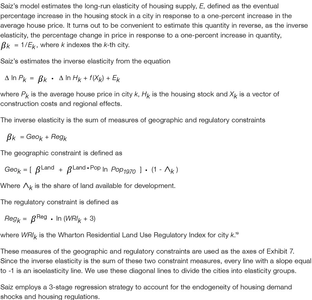
Saiz estimated a model of the long-run supply of housing that related house price changes between 1970 and 2000 to the measures of available land and the strictness of land use regulations described above.9 This model produces a numerical estimate of housing supply elasticity for each city in Saiz’s study.
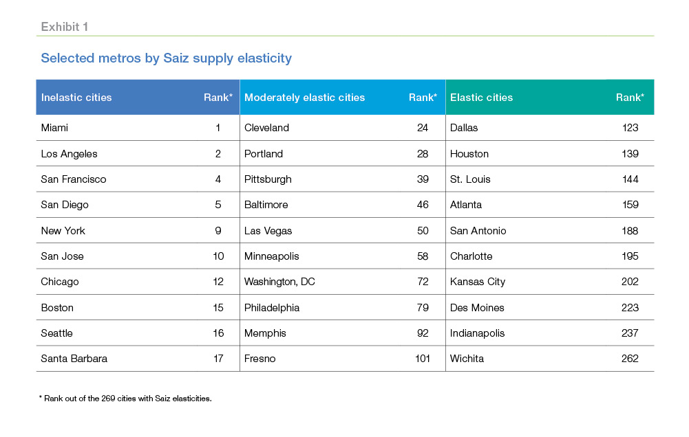
We use the Saiz elasticities to divide cities into three groups (Exhibit 1). In cities where the elasticity is less than 1.0, a one percent increase in the price of houses produces a smaller-than-one-percent increase in the supply of houses in the long run. These cities comprise the inelastic group. Cities with an elasticity greater than or equal to 1.0 but less than 2.0 comprise the moderately elastic group. And cities with elasticities of 2.0 or higher comprise the elastic group.
Cities in the inelastic group are much larger on average than cities in the other two groups (Exhibit 2). There are only 18 MSAs (containing 21 cities) in the inelastic group, but they contain over 25 percent of the U.S. population and have an average population of 4.6 million. There are 79 MSAs (87 cities) in the moderately elastic group (average population 1 million) and 156 MSAs (161 cities) in the elastic group (average population 570,000).
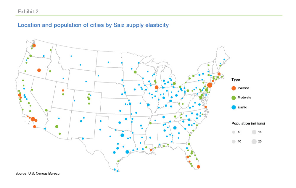
Except for Chicago, MSAs in the inelastic group are located near a coast.10 Eight are in California, five are in Florida, and the remainder are in Connecticut, Louisiana, Massachusetts, New York, Utah, Virginia, and Washington. MSAs in the elastic group are scattered primarily across Texas, the Midwest, and the East.
What difference does supply elasticity make?
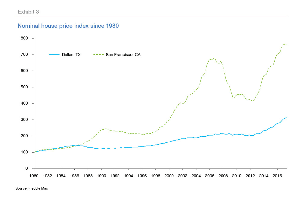
House prices are almost twice as volatile in the inelastic group of cities as in the elastic group. Increases in demand cannot produce much more housing, thus prices must adjust by a larger amount. Exhibit 3 compares the time path of an index of house prices in San Francisco, a city with inelastic housing supply, to the time path in Dallas, a city with elastic supply.11 House prices in San Francisco clearly have been more volatile than in Dallas.
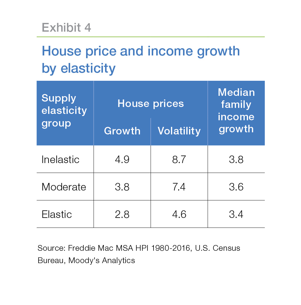
Not only have house prices been more volatile in inelastic cities, but house prices have grown 75 percent faster in inelastic cities than in elastic cities for the last 3-1/2 decades (Exhibit 4). However, growth in median family income has been only marginally higher in inelastic cities. As a result, cities like San Francisco, New York and Seattle have become more and more expensive, making it more and more difficult for middle-income workers to relocate to these high-growth areas.
The increasing cost burden of housing in the inelastic group of cities has limited their population growth despite their economic vitality (Exhibit 5). In 1970, the inelastic group of cities contained a higher share of the U.S. population than the moderately elastic or elastic groups. By 2002, the share in the elastic group of cities exceeded the share in the inelastic group. If current trends continue, the population share of the inelastic group may eventually fall below the share in the moderately elastic group as well.
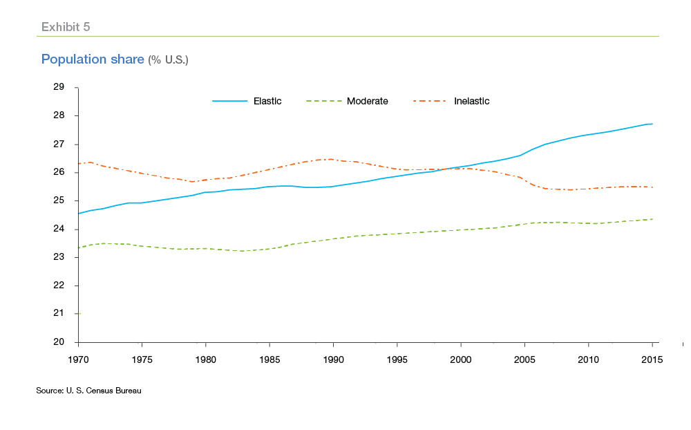
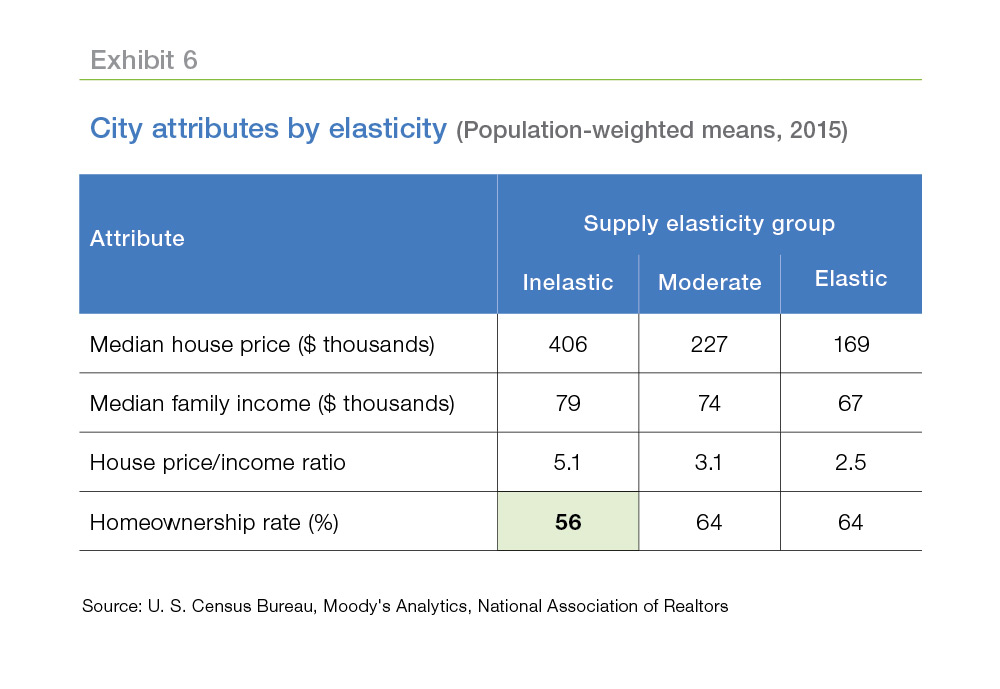
Exhibit 6 compares house prices, price-to-income ratios, and homeownership rates across the three elasticity groups. House prices in the inelastic group are 2.4 times higher than in the elastic group, and the house price to income ratio is twice as high. Most notably, the homeownership rate in the inelastic group is only 56 percent. Nationally, the homeownership rate hasn’t been that low since the 1950s.
Which matters more, regulation or geography?
Many scholars and policy makers have argued that reductions or refinements in land use regulations will increase the supply and lower the cost of housing, especially in high-growth, high-cost cities. The “Housing Development Toolkit” published last year by the White House recommended ten specific reforms to local land use regulations.13 However, for cities in the inelastic group, these proposals may not have as much impact as their sponsors anticipate.
All the cities in the inelastic group have significant geographic constraints. These constraints will continue to boost house prices and rents even if land use regulations are relaxed. Moreover, the scarcity of developable land increases the incentive for current homeowners to implement strict land use regulations to protect and further increase the values of their houses.
We can use the Saiz model of supply elasticity to estimate the relative impact of regulatory and geographic constraints on long-run house prices and to document the association between geographic and regulatory constraints. Exhibit 7 displays the combinations of land use regulations and geographic constraints—the key ingredients in the Saiz model—for the cities studied by Saiz.14 Increases in regulatory constraints (vertical axis) and geographic constraints (horizontal axis) both reduce supply elasticity, so elasticity is highest in the lower-left corner of the chart and lowest in the upper-right corner. The diagonal lines separate the cities into the inelastic, moderately elastic and elastic groups.
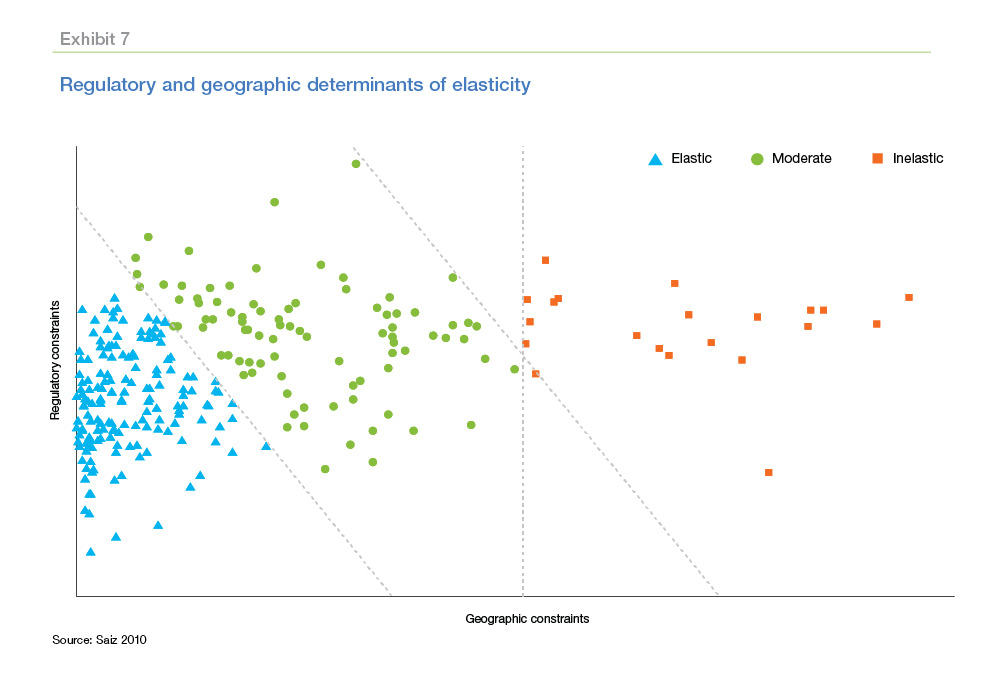
While both regulatory and geographic constraints combine to determine elasticity, inelastic cities can be identified solely by the level of geographic constraints. All the cities in the inelastic group appear to the right of the vertical line in Exhibit 7; each of these cities has a geographic constraint above the 92nd percentile of the values in Saiz’s sample. All the cities to the left of the line are in either the elastic or moderately elastic group.
Local land use regulations in inelastic cities are higher-than-average with little variation across cities.15 The limited variation in regulations in the inelastic group means that differences in supply elasticity among this group are determined by the level of geographic constraints alone. In contrast, regulatory constraints vary a lot within the elastic group. Cities in this group with negligible geographic constraints can have supply elasticities that vary by a factor of six.
Saiz argued that geographic constraints encourage cities to implement stricter land use regulations, an argument consistent with the pattern observed in Exhibit 7. According to this argument, population growth in a geographically-constrained city such as San Francisco increases house prices. Without regulation, price increases would be mitigated by new supply from developers. However, to protect the value of their homes, existing homeowners lobby for various limits to development, especially high-density development.16
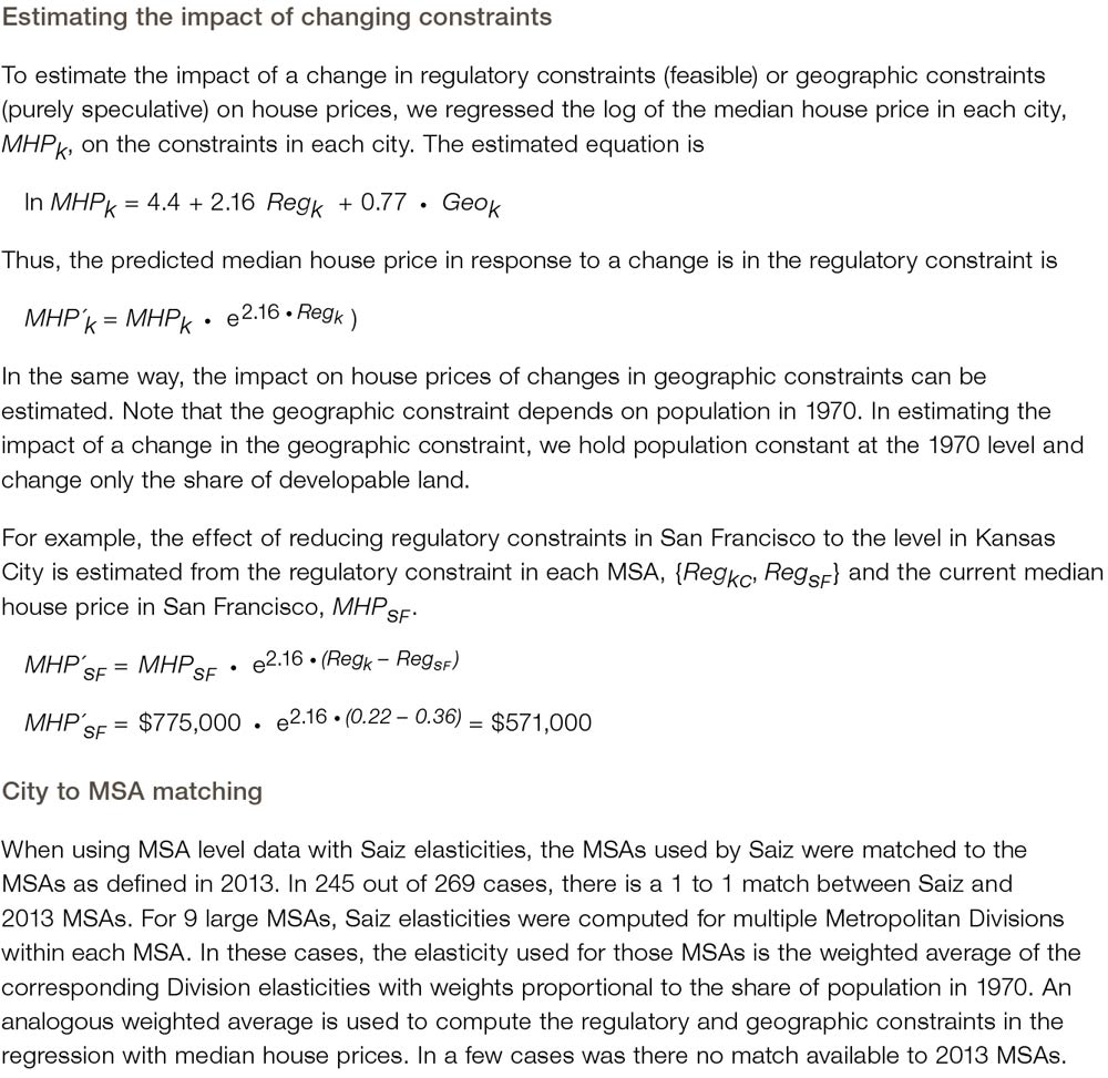
A thought experiment can illustrate the impact of regulatory relief and the limits on that relief in a city that also is constrained by geography. Imagine we could replace San Francisco’s current land use regulations with the regulations of the same strictness (same value of the Wharton index) as those in Kansas City. In this imaginary San Francisco, this regulatory relief would reduce the median house price by 26 percent, from $775,000 (2015 median) to $571,000.17 That substantial price drop is approximately the magnitude of the national price collapse in the housing crisis of the mid-2000s. It’s not surprising that existing homeowners would resist such a change in land use policies. However, even with a price drop of this magnitude, the median house price in San Francisco would still be more than 2.5 times higher than the national median house price.
The geographic constraints in San Francisco are, in fact, quantitatively more important than the regulatory constraints. Stretch your imagination a bit further and consider leaving San Francisco’s land use regulations unchanged but, instead, replacing San Francisco’s considerable geographic constraints with the almost-total lack of constraints in Kansas City. If this were possible18, the median house price in San Francisco would drop by an astonishing 54 percent in the long run to $359,000.
Advocates of regulatory reform often highlight the effects of strict regulations on cities like San Francisco, Seattle, Chicago and New York—all cities in the inelastic group and all cities with significant geographic constraints. And Saiz’s model suggests that reductions in regulation would lower house prices in these cities significantly in the long-run, although prices would remain higher than the national average. But, even if sufficient political momentum could be built to relax land use regulations, how likely is it that regulations would remain relaxed?
Imagine again that San Francisco’s land use regulations were relaxed significantly. The ensuing reduction in house values would encourage migration to San Francisco. However, the geographic constraints in San Francisco guarantee that housing would still be inelastically supplied despite the reduction in regulation. Over time, existing homeowners would find it more and more in their economic interest to lobby for the restoration of stricter regulations.
Both the impact and the likelihood of lasting regulatory reform appear to be limited by geographic constraints in cities with inelastic housing supply. For San Francisco, New York and similar cities, geography may be destiny.
However, California is considering a new approach that may succeed in permanently reducing or refining local regulations that restrict the supply of housing. California faces particularly severe housing affordability challenges. California contains more cities in the inelastic group than any other state, and even California cities in the moderately elastic group—cities like San Luis Obispo, Santa Cruz and Santa Rosa—have very high housing costs. The state Senate is considering “extraordinary legislation to, in effect, crack down on communities that have, in their view, systematically delayed or derailed housing construction proposals, often at the behest of local neighborhood groups.”
This state-level legislation, if it passes, may provide an avenue for implementing the types of proposals recommended in the White House’s “Housing Development Toolkit.” In addition, the passage of legislation at the state level may make it more difficult for local communities to reintroduce regulations designed to stymie development. While the impact of scarce land will continue to be felt, perhaps the double whammy of regulatory constraints on top of geographic constraints can be avoided.
Appendix
Prepared by the Economic & Housing Research group
Sean Becketti, Chief Economist
Elias Yannopoulos, Quantitative Analytics Professional
1 See, for example, "Housing Development Toolkit," The White House, September 2016 (https://obamawhitehouse.archives.gov/sites/whitehouse.gov/files/images/Housing_Development_Toolkit f.2.pdf), "Why is Manhattan So Expensive? Regulation and the Rise in Housing Prices," Edward L. Glaeser, Joseph Gyourko, and Raven Saks (http://repository.upenn.edu/penniur_papers/8/), and "The Economic Implications of Housing Supply," Edward L. Glaeser and Joseph Gyourko, Zell/Lurie Working Paper #802, January 4, 2017.
2 Hsieh, Chang-Tai and Enrico Moretti, "Housing Constraints and Spatial Misallocation," NBER Working Paper 21154, revised May 2017, http://www.nber.org/papers/w21154. Bunten (2017) also examines the welfare cost of zoning regulations and estimates an impact about half that of Hsieh and Moretti. Bunten, Devin (2017) "Is the Rent Too High? Aggregate Implications of Local Land-Use Regulation," Finance and Economics Discussion Series 2017-064. Washington: Board of Governors of the Federal Reserve System (https://doi.org/10.17016/FEDS.2017.064). In addition, the "Housing Development Toolkit" notes that these types of regulations and the associated high housing costs (a) reduce jobs in construction and related fields; (b) reduce nimbleness in adapting to shifts in economic conditions; (c) push many working families further and further out from the city and increase commute times and costs, with associated environmental impacts such as increased gas emissions; and (d) increase the cost of public housing assistance resulting in a reduction of the number of households served.
3 See Gyourko, Joseph, Albert Saiz, and Anita A. Summers “A New Measure of the Local Regulatory Environment for Housing Markets: The Wharton Residential Land Use Regulatory Index,” Urban Studies, 45 (2008), 693-729. The WRI is a composite index of 11 sub-indices, each of which captures a different dimension of the various forms of land use regulations.
4 Formally supply elasticity measures the percentage change in the supply of a good in response to an increase in demand that raises the price of a good by one percent. Demand elasticity measures the percentage change in the quantity demanded of a good in response to an increase in supply that raises the price by one percent. In this article, we focus on the supply elasticity of housing.
5 Perhaps some non-housing examples may make the concept of elasticity clearer. Leonardo da Vinci’s painting the Mona Lisa is an example of a completely inelastic good. No matter how much the price increases, there will be no increase in the supply of (authentic) Mona Lisas. In contrast, the supply of radishes is highly elastic. Radishes grow quickly, they are small, easy to ship, and growable in a wide variety of environments. If scientists discover that consuming large quantities of radishes will keep you young or help you lose weight, farmers will boost supply in short order, but prices will change little.
6 Saiz computed elasticities at a city level. The “city” is defined as a circle with a 50-kilometer radius around the city center. In this article, we switch between city-level and MSA-level analysis freely. We developed an algorithm for matching cities to MSAs, which allows us to combine elasticities for multiple cities within a single MSA.
7 Saiz used digital contour maps to estimate the area lost to oceans and the Great Lakes. The area covered by wetlands or with grades greater than 15° is derived from United States Geological Survey data.
8 Low availability of developable land is a constraint only if the population is large enough for the land constraints to bind. Accordingly, Saiz included the interaction between the population in 1970 and the share of undevelopable land in the estimation of housing supply elasticity.
9 The Saiz model controls for changes in construction costs and regional effects as well, but the impacts of regulation and land availability are the key factors in determining housing supply elasticity. See the appendix for an overview of the Saiz housing supply model.
10 And Chicago is located on the coast of Lake Michigan.
11 The indices for both cities are normalized to 100 in 1980 to facilitate comparison.
12 The shares add up to less than 100 percent, because Saiz estimated elasticities for only 269 U.S. cities.
13 Recommendations include establishing by-right development; taxing vacant land or donating it to non-profit developers; streamlining or shortening the permitting processes and timelines; eliminating off-street parking requirements; allowing accessory dwelling units; establishing density bonuses; enacting high-density and multifamily zoning; employing inclusionary zoning; establishing development tax or value capture incentives; and using property tax abatements.
14 See the appendix for a description of how regulation and geographic constraints are derived from the Saiz model. The regulatory and geographic factors measured on the axes of Exhibit 7 combine raw data on the WRI, the share of unavailable land, and population with estimated coefficients from the Saiz model in a way that makes it possible to use diagonal lines as separators of elasticity zones.
15 New Orleans stands apart from the other cities in the inelastic group. It is the only city in the group with well-below-average regulatory constraints. However, its geographic constraints are so severe that it would be in the inelastic group if it had no regulatory constraints, as measured by Saiz.
16 Glaeser and Gyourko (2017) point out that the concentrated economic interests of existing property homeowners generally are much higher than the pro rata benefits to potential homebuyers and renters, making it difficult to mobilize political support for relaxing land use regulations. In addition, high housing costs prevent many potential beneficiaries from moving to high-cost cities, hence disqualifying them from voting in the affected area.
17 See the appendix for a description of the calculations in this example.
18 Small changes in land availability are possible. Foster City in San Mateo County—one of the five counties in the San Francisco Bay area—was built on engineered landfill in the marshes of the San Francisco Bay. Currently it is home to almost 35,000 people.