


The Housing Supply Shortage: State of the States
The United States suffers from a severe housing shortage. In a recent study, The Major Challenge of Inadequate U.S. Housing Supply, we estimated that 2.5 million additional housing units will be needed to make up this shortage. Our earlier study used national statistics, treating the United States as a single market. What happens when we look closer, basing the analysis at the state level?
When we account for state-level variations, the estimated housing deficit is even greater in some states because housing is a fixed asset. A surplus of housing in one area can do little to help faraway places. For example, vacant homes in Ohio make little difference to the housing markets in Texas. We estimate that there are currently 29 states that have a housing deficit, and when we consider only these states, the housing shortage grows from 2.5 million units to 3.3 million units.
Unsurprisingly, the states with the most severe housing shortage are the states that have recently attempted to loosen zoning policy regulations. States like California, Oregon, and others have undertaken policy action to address this issue. California, for example, has been working on chipping away at single-use zoning while Texas has passed a density bonus program, an ordinance which amends the city code by loosening site restrictions and promoting construction of more units in affordable and mixed-income housing developments. Oregon was one of the first states to pass legislation to eliminate exclusive single-family zoning in much of the state. The Minneapolis City Council voted to get rid of single-family zoning and started allowing residential structures with up to three dwelling units in every neighborhood. We took a deep dive into the supply/demand dynamics to analyze state-level variations.
We estimate that there are currently 29 states that have a housing deficit, and when we consider only these states, the housing shortage grows from 2.5 million units to 3.3 million units.
Accounting for housing supply/demand conditions
To estimate housing supply, we rely on U.S. Census Bureau estimates of the total number of housing units in each state. These estimates include single-family homes, apartments, and manufactured housing. We compare supply to our estimates of housing demand. We first focus on static estimates of housing demand, and then we consider the impact of interstate migration.
Our estimate of housing demand relies on two components. First, we need an estimate of long-term vacancy rates ( v* ). Second, we need an estimate of the target number of households ( h* ). 1 The estimates of v* and h* give an estimate of housing demand ( k * ) using the formula:
Vacancy rates
As we discussed in our earlier study, for the housing market to function smoothly, year-round vacant units are needed. Vacancy rates are often used to track the vitality of the housing market. Too high of a vacancy rate reflects a moribund market, while too low of a rate means demand is outstripping supply. Our previous research estimated the average U.S. vacancy rate to be around 13%.
For long-term vacancy rates ( v* ), we use historical estimates of vacancy rates in each state as well as the share of the state in the housing stock to obtain the state weight. We compute the weighted average national vacancy rate for the U.S. and then estimate the deviation of the state vacancy rate from the average national vacancy rate (see Appendix 1.1 for a detailed methodology). We use each state's average from 1970 to 2000 as the estimate for v * because this was the period before the boom and the bust in the housing market began. Historical vacancy rates vary dramatically by state. States like Vermont and Maine tend to have high vacancy rates because a large fraction of the housing stock serves as vacation/second homes. On the other hand, states like California tend to have very low vacancy rates.
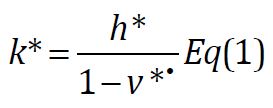
It is interesting to compare each state’s long-term vacancy rate ( v * ) to recent estimates ( v ). This measure estimates the number of housing units needed to close the gap between the current vacancy rate and long-term average rates. Exhibit 1 shows the difference between the estimated vacancy rate in 2018 and the long-term vacancy rate for each state. States like Oregon, California, and Minnesota have much lower current vacancy rates compared to their historical averages, while states like West Virginia, Alabama, North Dakota, and Ohio have witnessed an increase in the vacancy rates as the populations of these states have decreased.
Target households
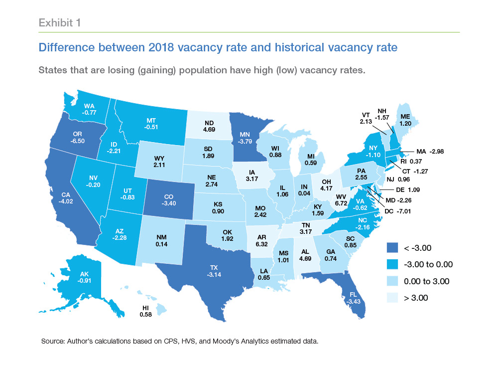
Our previous research has shown that high housing costs have constrained household formation. These high housing costs have hit the Millennial generation particularly hard. To overcome these cost barriers, some young adults have turned to shared living arrangements. Others have moved back home with parents. As a result, there are more than 400,000 missing households headed by 25- to 34-year-olds (households that would have formed except for higher housing costs).
While high housing costs have hit young adults hardest, they have affected all age groups. If housing costs were lower, more households would form. We use our model estimates of the number of households reduced due to unusually high housing costs and add them back. We do this for each age group (see Appendix 1.2 for more details.) Due to different age profiles, the share of missing households varies by state. Exhibit 2 plots the share of missing households due to housing costs for each state. In general, states with relatively lower vacancy rates have proportionally more missing households.
Static estimate of housing deficit
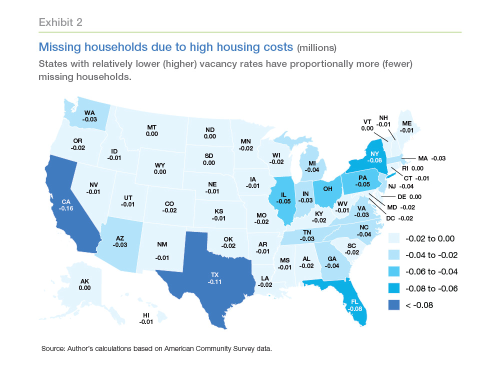
We combine our target vacancy rate and target households to estimate housing demand. Subtracting our estimated housing demand from the Census estimate of housing supply gives us the estimated housing deficit. Exhibit 3 shows our results by state.
As a percent of the housing stock, the state housing supply deficit varies from -7 to 10%. Excluding the District of Columbia, Oregon has the largest deficit (nearly 9%) followed by California (nearly 6%).2 Some states have a negative deficit, meaning they are oversupplied. According to our estimate, 21 states are oversupplied, the largest being West Virginia, at more than 7%.
Impact of migration on the housing deficit of the states
While houses stay in place, people do not. Job growth attracts in-migrants, while a dearth of opportunity drives out-migration. High housing costs also contribute to migration patterns. When the rents get too high, people move away. This dynamic can impact our estimates.
It's helpful to consider the case of California. Our estimates indicate that California has a shortage of 820,000 housing units. But history suggests that California's shortage may be overestimated if interstate migration is considered. For more than four decades, California's state population has grown, but this increase has been driven primarily by international migration. High housing costs have driven many U.S. citizens and households out of California, driving housing demand higher in their destination states.
A robust model of domestic migration flows between states is beyond the scope of this study. But we can approximate how migration may affect our estimates. We can use the historical average of state-to-state migration flows as a forecast of future flows. If the future interstate migration exactly matches past flows since 2001, we can create a rough, but useful approximation (Exhibit 4).3
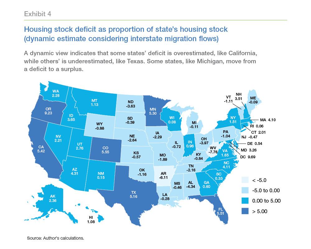
For example, when considering migration flows, the estimated housing demand in Michigan changes from deficit to surplus; Ohio's surplus increases; and Florida’s deficit increases (see Appendix 1.3 for details on our estimation method).
Given the severity of the problem, states have started addressing the issue of supply shortages by taking legislative action. Some of these states such as California, Oregon, Minnesota, and North Carolina have passed legislation to eliminate exclusive single-family zoning. Removing these zoning restrictions will provide builders with the flexibility to build a range of housing options which could help alleviate some of the shortage.
Conclusion
A shortage of housing remains a major issue for the United States. Years of underbuilding has created a large deficit, particularly for states with strong economies that have attracted a lot of people from other states. The issue of undersupply will be further exacerbated as Millennials and younger generations enter the housing markets.
Dynamic estimates suggest that contrary to expectations, it isn’t only the larger states that have a higher housing supply shortage. Some of the smaller states, which have been attracting a lot of migrants from other states, also need to build more housing units to accommodate the needs of their growing population.
Appendix
1.1 Vacancy rate calculations
We calculate the vacancy rate based on the historical vacancy rate. For this purpose, we obtain the historical vacancy rates by state from Moody’s analytics for the period from 1970 to 20004 and estimate the average vacancy rate for this period for each state.
for 1970–2000, where
is the state.
We then obtain the housing stock information by state from the Housing Stock (HVS) ('000s) U.S. Census Bureau (BOC): Housing Vacancies and Homeownership–Table 8–Quarterly Estimates of the Housing Inventory. From these data, the share of the state in the total housing stock is calculated to get the state weights.
The sum product of the vacancy rate of the state and the state’s weight in the housing stock gives us the U.S. average vacancy rate. U.S. average vacancy rate:
.
We then compute the difference between the state vacancy rate and the average U.S. vacancy rate to see how far away the state is from the U.S. average.
This deviation for the states is then applied to the long-run vacancy rate for the United States (which we estimated earlier to be 13%) to get the state-wise vacancy rate.
State-wise Vacancy Rate = 13% +

for each state.
1.2 Estimating target households
We obtain the headship rates5 for the year 2018 by state and by age for all the 50 states and District of Columbia.6 We then estimate target households using this headship rate and adding back housing costs assuming that housing costs become more favorable for household formation.
The target headship rate would be
.
We then use this target headship rate and the population by five-year age buckets to compute the households in each state.
where
is the state and

is the five-year age buckets.
The product of headship rate and population by age gives the households by age group. Summing it up over all the ages gives the total households in the state.7
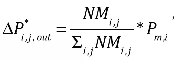
1.3 Domestic migration flows between states
For the estimate of the states’ share of the deficit, we need to obtain the share of the migration flows between states by age. To get detailed age-wise distribution of population, we use the ACS data from 2001 to 2017. We obtain the population by age and by state for these years. We identify people who had a different state of residence from a year ago, which indicates that they migrated to a different state. We then get estimates of the in-migrants and out-migrants by state and age.
We then estimate the net domestic migrants for each state as the difference between the in-migrants and out-migrants.

where i is the state, j is the five-year age buckets, I is the in-migrants, and

is the outmigrants.
To estimate the net outmigrants from states that have a
, we obtain the Moody’s historical net domestic migration data. We then apply these shares by state and age to the net migration data for 2018 to obtain the number of people leaving a state by the five-year age bucket.
where
is the total change in population (net out-migrants) for states that have net outmigration,
is the net out-migrants by age group and state,
is the sum of the total out-migrants for the state, and
is the historical net domestic migration data from Moody.
The ratio of

gives the share of the five-year age group in the total out-migrants from the state.
This pool of out-migrants
is then divided among the in-migrating states, given that the net flows for the country are

.
We distribute these migrants according to the share of the state in the total in-migrants as well as by the share of the age group in the total in-migrants to the state.
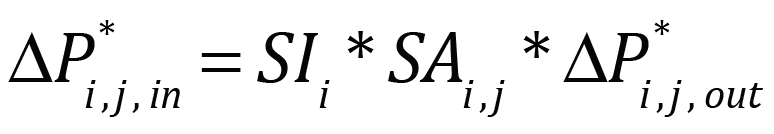
where
is the in-migrants to the state i from the outmigrants pool,

is the share of the state in total in-migrants,

is the share of the five-year age bucket in the total in-migrants, and
is the total out-migrants.
The population of each state is then adjusted according to the change in the population estimated above.
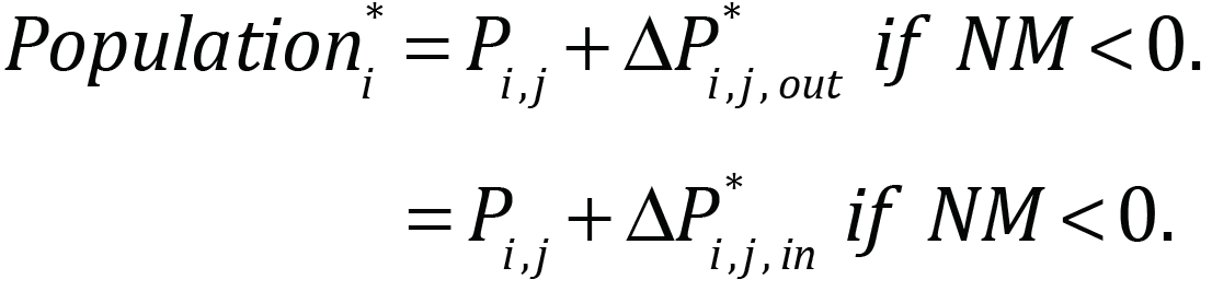
The households are then computed based on this adjusted population for each state by applying the headship rates by age group. Then the housing stock is estimated as per equation (1).
Prepared by the Economic & Housing Research group
- Sam Khater, Chief Economist
- Len Kiefer, Deputy Chief Economist
- Venkataramana Yanamandra, Macro Housing Economics Senior
- The target number of households is the number of unconstrained households that would have formed if households did not face any constraints related to housing costs.
- The District of Columbia had the highest deficit as a share of the existing housing stock at 9.7%.
- We used the average net migration flows between states from 2001 to 2017 for the past flows.
- Data is available from 1970:Q2 onward. We estimate the average for the period up to 2000:Q4. This corresponds to the period before the boom and bust in the housing market began.
- Headship Rate = Number of Head of Households/Total Households.
- Data source: Current Population Survey–Annual Social and Economic Supplement (CPS-ASEC) using the Integrated Public Use Microdata Series (IPUMS) (Steven Ruggles, Sarah Flood, Ronald Goeken, Josiah Grover, Erin Meyer, Jose Pacas and Matthew Sobek. IPUMS USA: Version 9.0 [dataset]. Minneapolis, MN: IPUMS, 2019.)
- These households would be based on the Current Population survey (CPS). To make them consistent with estimates of housing supply from HVS, we apply a multiplier to this gap that is proportional to the gap between the CPS-ASEC and HVS household counts. The CPS-ASEC household estimate for 2018 was 127.6 million. The HVS estimate for that year was 121.3 million. We deflate our target households by a factor equal to 121.3/127.6, or 0.95.