U.S. Population Growth: Where is housing demand strongest?

What is the main driver of demand for housing in the United States? The answer is simple: people. The American population is a diverse group with multifaceted and individualistic housing needs. Housing is a long- lasting investment, so investment decisions made today in the type of housing built will shape the availability of housing long into the future. The slow-moving currents of housing demand and supply are often distorted in the short run by economic factors such as the business cycle or interest rate movements. But in the long run, the deep forces of supply and demand, including demographic-driven demand, shape the housing market, the cost of housing, and ultimately, who lives where and in what type of housing.

Our understanding of the long-run demand for housing in the U.S. comes from the careful study of detailed historical data on the demographics of the American people. Precisely, because absent calamity, the nation’s population changes slowly. Despite slow changes, factors such as shifting mortality and immigration lead to surprises in housing demand trends. Gradually, new construction arises to replace deteriorating housing stock and accommodate new households. Overall, in the past decade, housing supply has failed to match the undercurrents of demographic-driven housing demand for various reasons (such as lack of labor, land-use regulation, rising raw material costs, and lack of available lots for development). The result has been intense pressure on rents and house prices, whose growth has far outpaced the price growth of non-housing goods and services.

These dynamics play out in the thousands of individual housing markets that make up the United States. The American people continue their slow migration toward Southern and Western states. As they empty the great industrial cities of the North and Midwest, these domestic migrants compete for housing with the influx of migrants from abroad seeking economic opportunity in America. In the South and West, and in the remaining vibrant markets of the Midwest and Northeast, new families and new generations face fierce competition for housing not only from others of their own age cohort and international migrants, but also an aging population that is living longer, healthier lives and is aging in place. Many of the fading industrial cities face an overabundance of housing and declining population accelerated by job loss, out-migration, and the aging of their remaining inhabitants.

Risks on both sides of the housing market are rising. Specifically, in hot, growing markets, the undersupply of housing is leading to speculative booms. Conversely, in contracting markets, oversupply (mostly driven by a shrinking population) is leading to a slowdown in house price appreciation.

Freddie Mac has a keen interest in understanding not only how recent demographic trends have unfolded, but also how those trends will shape the future of housing demand and supply. Our mission to provide liquidity, stability, and affordability to the nation's housing markets can be accomplished only with an understanding of the forces driving housing markets. We have recently published several research studies and Insights examining these forces, but much work remains to enhance our understanding. To understand the future, we need to understand the longer-term changes that have been taking place with respect to demographics. Specifically, we look at which regions and metro areas have been gaining population. Furthermore, we look at what factors are driving these geographic trends. By looking at these trends, we can better understand where the housing demand is likely to come from in the future.

Slowdown of U.S. Population Growth

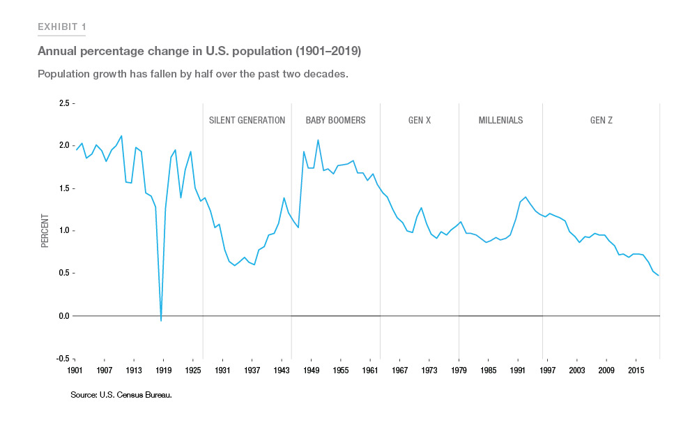
U.S. population has been slowing for decades, but the slowdown has been more pronounced in recent years. Exhibit 1 shows the annual population change in the U.S. from 1901 to 2019. As of 2019, the annual population growth rate was the lowest since 1918 at 0.48%, down from an average of 0.54% in the 3 years from 2017 to 2019 and 0.83% in 2010. The slowdown in the annual population growth rate was driven by declining natural increase (birth rates contributing 22%, death rates contributing 7%) and declining net migration (contributing 71%). The COVID-19 pandemic may have a negative impact on the birth rates while pushing up the death rates, leading to an even slower population growth in 2020.¹

Starting in the 1940s, the Baby Boomer cohort (those born between 1946 and 1964) drove population growth. From the 1950s to the 1970s, population growth rates steadily declined. The trend was reversed with the rise of the Millennial generation (1981–96). In fact, as of 2019, Millennials surpassed Baby Boomers to become the largest cohort. However, since the mid-1990s, population growth has again slowed.

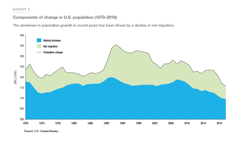
Three components make up the total change in a population: births, deaths, and net migration. Fertility rates for the native-born population have been declining for more than a century. Births per 1000 population declined from 30 in the early 20th century to 25 by mid-century and had fallen to just 11.5 as of 2019. Death rates per 1,000 population fell from 1950 until 2010 but are now slowly climbing as the U.S. population ages. U.S. population increased by 1.5 million in 2019, as a result of 3.8 million births, 2.8 million deaths, and net international migration of 0.6 million (Exhibit 2).

In addition to a slowdown in the natural increase of population, a recent slowdown in net migration could have significant implications on housing demand in the near future. Specifically, from 2017 to 2019, net migration has fallen nearly 40%. This can be mostly attributed to tougher international migration restrictions. As a result of tepid net migration, the Census population estimate for 2020 is about 2 million less than what the Census had forecasted for 2020 three years ago. Even as declining birth rates and net migration slow the overall U.S. population growth, recent domestic migration patterns towards the southern and western parts of the U.S. mean housing markets in these regions are seeing strong growth in recent years.

Migration South and West

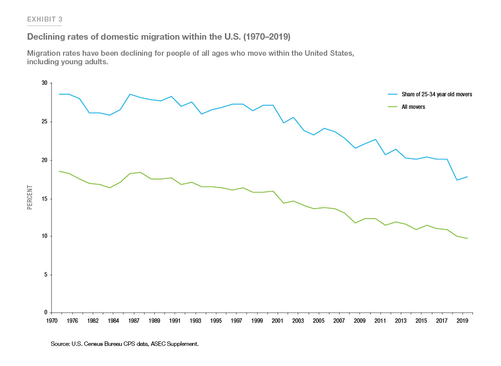
Migration, both into and within the country, has been a perennial characteristic of U.S. demographics. However, migration rates within the U.S. have been declining for many years, with the lowest migration rate on record at 9.8% during 2018–19. This decline is occurring not only among older Americans, but even among Millennials who are moving less often than they used to (Exhibit 3). The share of movers in the 25–34 year range has declined from approximately 30% in 1970 to less than 20% in 2019.

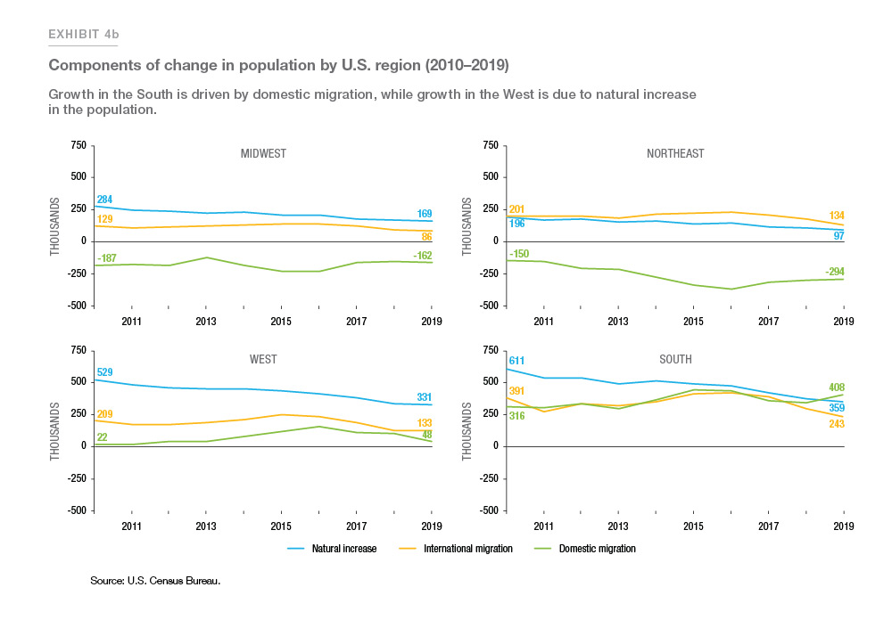
From a regional population growth perspective, the South led the way in 2019 with year-over-year growth of 0.81%, followed by the West (0.66%), the Midwest (0.14%), and the Northeast (-0.11%). From 2017 to 2019, population in the South and West grew at around seven times the rate of growth in the Northeast and Midwest (Exhibit 4a).

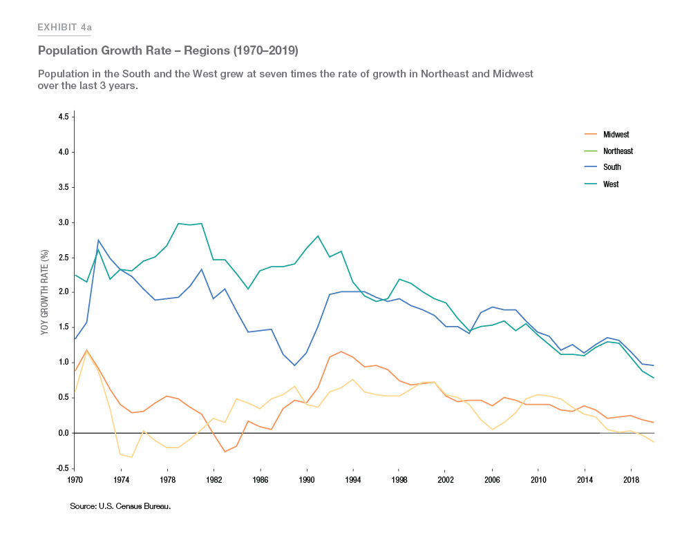
If we break up each region by components of change, we see outmigration occurring in the Midwest and Northeast. Take this outmigration and add a slow down in natural growth and you get a decline in overall population for these two regions. It is noteworthy that the two regions experiencing the fastest growth – the South and West—have different drivers of population growth. In the West, population growth is driven mostly by natural increase from the younger population in the Rocky Mountains, while in the South, population growth is mainly driven by domestic migration (Frey, (2018); Felix et al (2018); Kerns & Locklear (2019)).² For example, Texas has been attracting young adults in their prime working age and Florida is a retirement destination that attracts more seniors (Exhibit 4b).

Population trends within metro areas

A closer look at trends in Metropolitan Statistical Areas (MSAs) offers insights into local housing markets.

Population growth (absolute growth)

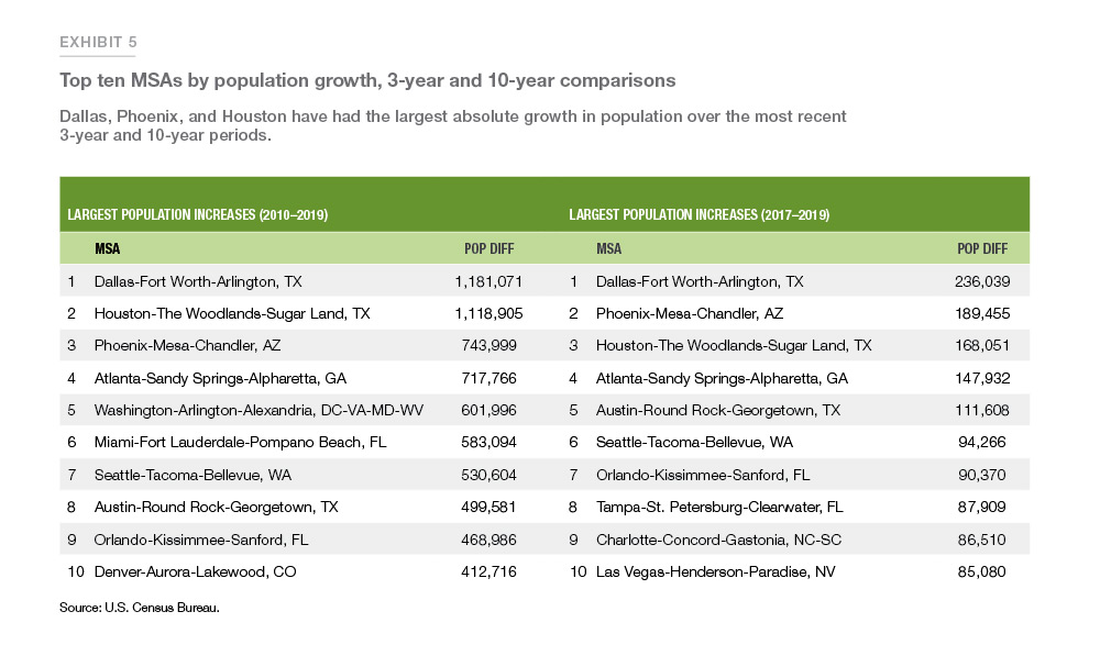
Over the last decade, population in absolute numbers increased the most in multiple MSAs within Texas and Florida. Specifically, population in three MSAs in Texas grew by a combined total of 2.8 million: Dallas (1.2 million), Houston (1.1 million), and Austin (0.5 million). Similarly, two MSAs in Florida accounted for a population increase of slightly more than 1 million: Miami (0.6 million) and Orlando (0.5 million). Favorable weather, lower cost of living, and the growing economies with increased job opportunities have attracted a lot of talent to these two states over the last decade. A comparison of the absolute growth in population over 3 years (2017 to 2019) and 10 years (2010 to 2019) shows that Houston, TX has fallen in ranking in recent years, along with Washington, DC and Miami, FL which are no longer in the top 10 (Exhibit 5). Meanwhile, Austin, TX, Seattle, WA, and Orlando, FL, have been gaining population, along with Tampa, FL and Charlotte, NC MSAs.

Population growth (percentage growth)

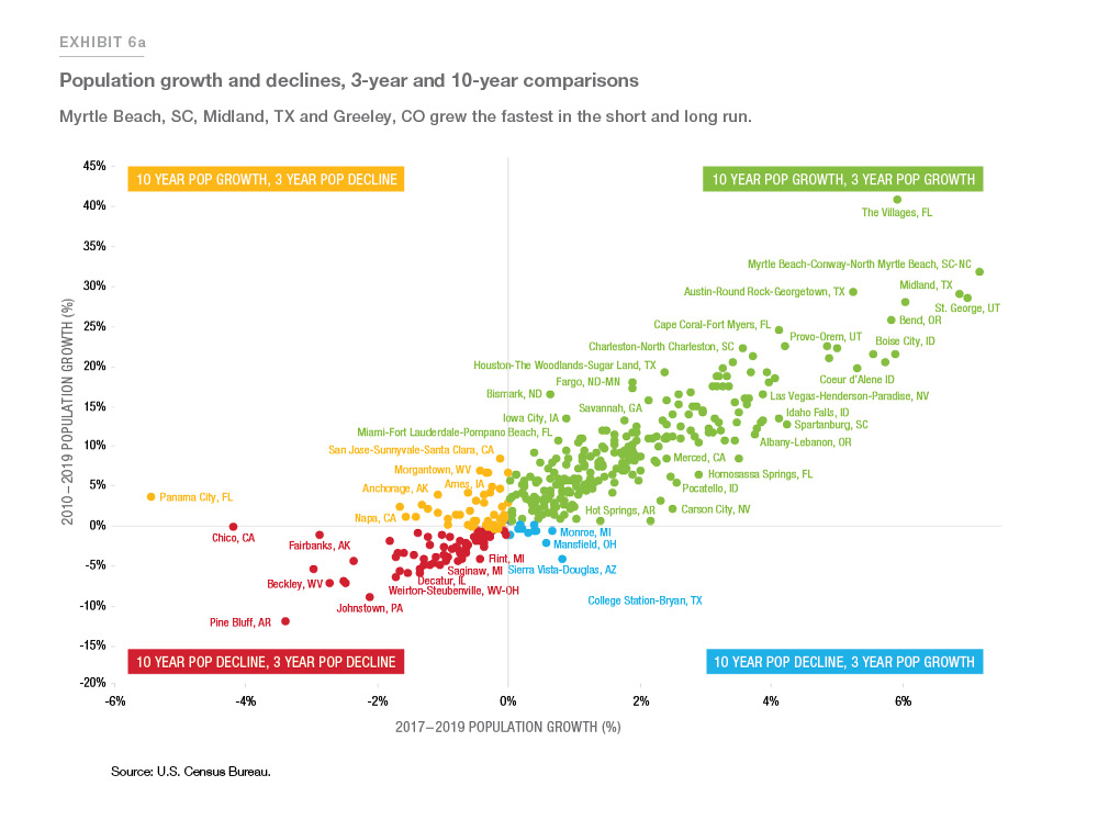
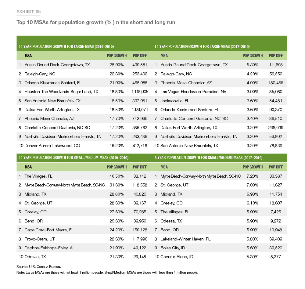
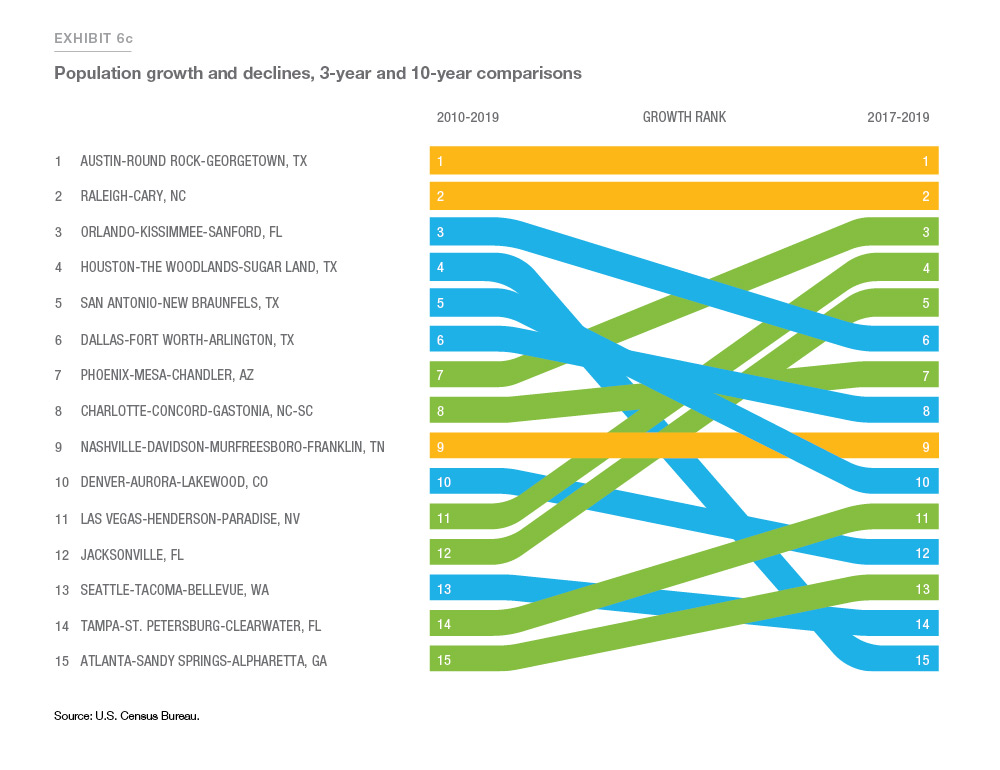
A look at the top MSAs by population growth in percentage terms shows slightly different trends than when we look at absolute numbers. In terms of the past 10-year percent growth, the top MSAs with the fastest growth are The Villages, FL (40.5%), Myrtle Beach, SC (31.3%), Austin, TX, (28.9%), Midland, TX (28.8%), St. George, UT (28.3%), Greeley, CO (27.6%), and Bend, OR (25.3%). In fact, Myrtle Beach, SC (7.2%) was the fastest growing MSA in the past 3 years followed, by St. George, UT (7.0%), Midland, TX (6.9%), and Greeley, CO (6.1%) (Exhibit 6a & 6b). Houston, TX, San Antonio, TX and Orlando, FL fell in rank in percent terms while Phoenix, AZ, Jacksonville, FL and Las Vegas, NV have gone up in rank. (Exhibit 6c).

Components of change

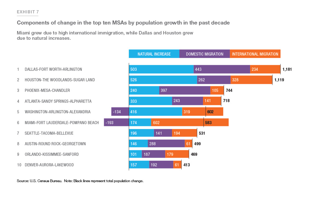
Comparing the components of population change for the 10 fastest growing MSAs, we can see that over the last 10 years, population everywhere except in the Washington, DC MSA was mainly driven by net migration. The Washington, DC metro predominately grew because of natural increase (more births than deaths) (Exhibit 7).

In terms of migration, Orlando, FL had the highest net migration rate, with 78% of the population growth coming from migration, equally distributed between domestic and international migration. Miami, FL, Austin, TX, and Phoenix, AZ also had high net migration. In absolute numbers, the MSA with the largest number of international migrants was New York.

Most of the population increase in the top 10 MSAs had been due to net migration both in the long and short runs. Houston, TX was the only exception, in that it had different factors driving long run and the short run change: the long-run driver had been migration, while the short-run driver had been natural increase.

City versus suburb: Where are people moving?

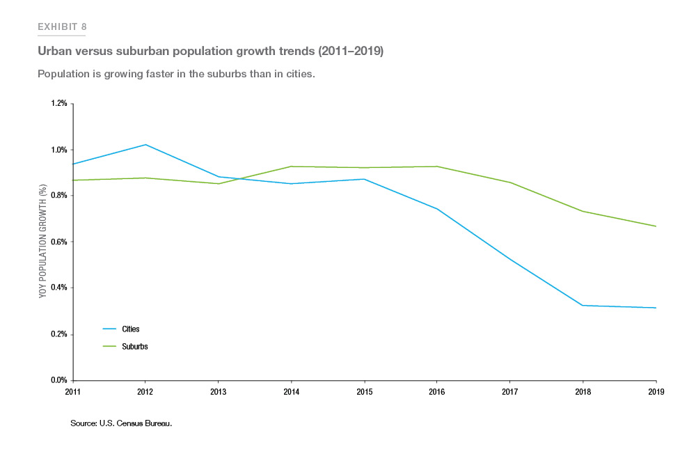
Another trend for the country as a whole over the past few years has been the movement toward the suburbs and away from the cities (Exhibit 8). In 2019, the suburbs grew at an annual growth rate of 0.7% while cities grew at half the rate (0.3%). This trend could intensify during the current pandemic, though it is too soon to declare the pandemic as a catalyst for a permanent trend in preferences.³

The aging Millennial cohort is contributing to this trend as members reach various life events such as getting married and having children. Thus, they are seeking larger homes and amenities, such as good schools. Which MSAs have contributed to this trend? And are any patterns emerging across regions?

As previously discussed, the fastest growing cities (in absolute terms) are mostly concentrated in the Southern and Western states. Phoenix, AZ, Houston, TX, San Antonio, TX, Los Angeles, CA, and Austin, TX are among the top ten urban areas that have experienced the most population increases. Columbus, OH is the only Midwestern city to make it to the top fifteen in terms of population growth between 2010 and 2019 and to the top ten in terms of population growth between 2016 and 2019. In fact, Columbus, OH gained more population than cities like Washington, DC and Jacksonville, FL. The city has received a lot of in-migration from within Ohio, while the overall growth of population in Ohio has been stagnant.

Another interesting case is Philadelphia, PA which has often been considered one of the declining legacy cities in the Northeast (Berube, 2019).⁴ The city gained more population over the period from 2010 to 2019 than cities such as Orlando, FL, that had been among the fastest growing markets. Another city that was on the decline but has turned around is Oklahoma City, OK. It witnessed a larger increase in population over the last 10 years than big cities like Boston, MA, Miami, FL, and San Jose, CA. In percentage terms, Frisco, TX has gained the most population: 70% over the last 10 years. South Jordan City, UT and Meridian City, ID are among the top ten cities growing at the fastest pace.

To study the growth between cities and suburbs, we divided each MSA into its cities and suburbs (Exhibit 9).⁵ We classified MSAs into four quadrants:

• Cities and suburbs are both growing
• Cities and suburbs are both declining
• Cities are growing and the suburbs are declining
• Suburbs are growing and the cities are declining

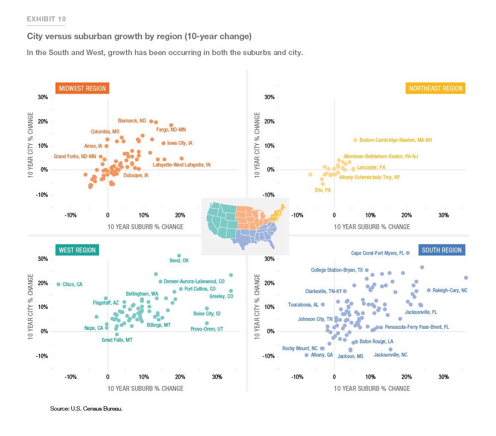
We find that 60% of the MSAs had faster suburb growth than city growth. Additionally, most MSAs fall in the top-right quadrant, where both cities and suburbs are growing. Interestingly, in some of the fastest growing places such as Boise, ID and Provo-Orem, UT, we find that the suburbs are growing faster than the city, while in areas such as Cape Coral, FL, Midland, TX and Bend, OR, the growth is taking place in the cities as compared to the suburbs. Most of the MSAs in Texas are witnessing a faster growth in suburbs than in the cities. On the other hand, places such as Baltimore, MD are witnessing declining city growth along with increasing suburban growth. Chico, CA stands out as the only place that has high city growth and declining suburb growth. This trend has been mainly attributed to resettlement in the city following the rising wildfires in neighboring areas (Wade, 2019).⁶

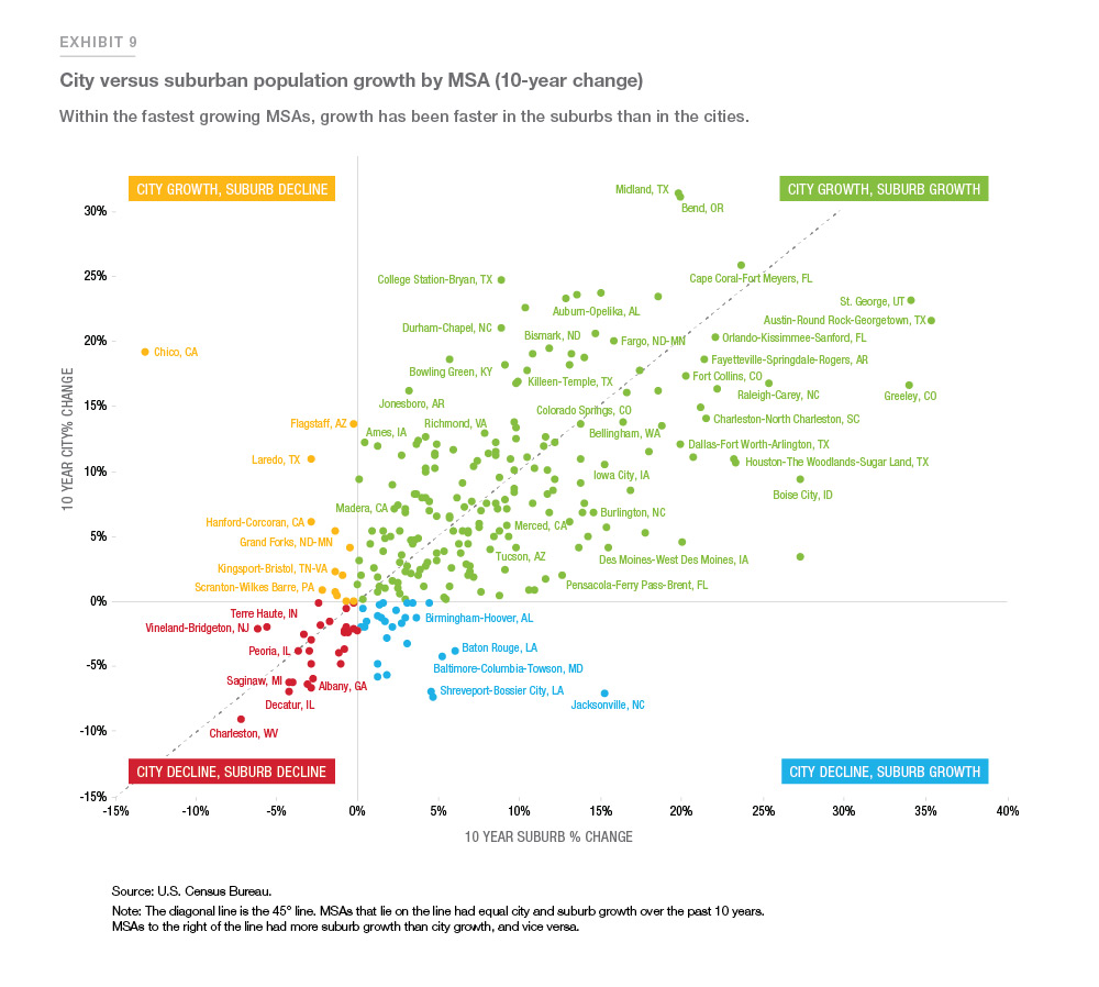
Exhibit 10 examines the city-suburb divide by region. Both city and suburban growth are increasing in most of the Southern and Western MSAs, while both are decreasing in most Northeastern MSAs.

How much does population change contribute to house prices?

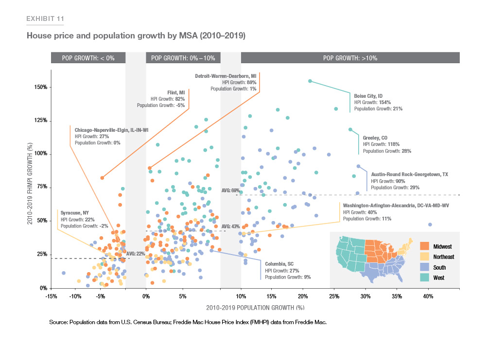
Exhibit 11 presents a scatter plot of house price and population growth between 2010 and 2019. The regional concentration in the South and West is apparent. While Exhibit 11 shows that the average house price growth is higher in MSAs with higher population growth, our analysis (discussed below) yields slightly different results. This is because there are other factors, such as housing stock and incomes that also affect house price appreciation.

While a detailed analysis to understand the impact of population increase on house prices is beyond the scope of this Insight, we did a simple decomposition analysis. The analysis looked at the impact of changes in population, per capita incomes, and per capita housing stock on the change in the median house prices between 2010 and 2019.

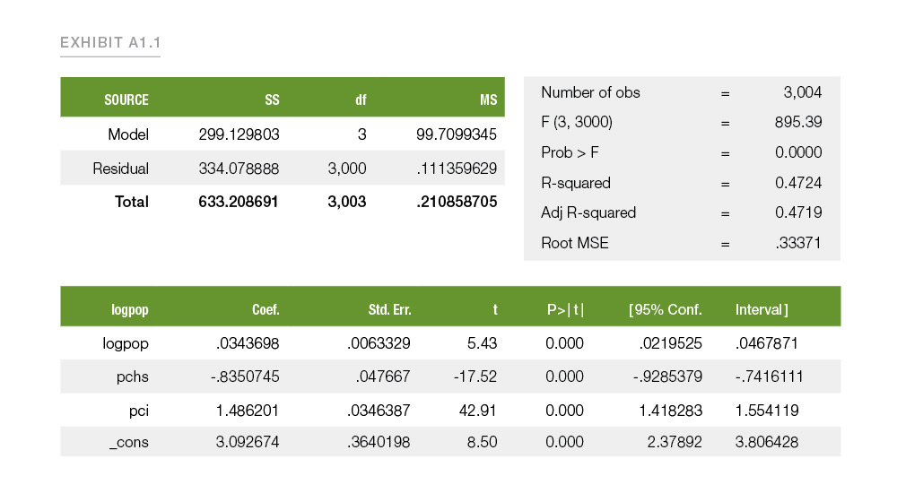
A simple regression analysis suggests that population change does not have a direct impact on house prices (see regression results in Appendix 1). The analysis suggests that a 1% increase in population increases house prices by 0.03%. Conversely, a 1% increase in per capita housing stock (housing stock/population) reduces house prices by 0.83%. Per capita income (income/population) has the most impact on house prices, with a 1% increase in per capita incomes leading to a 1.5% increase in house prices. These results are in line with what has been observed in the literature (for example, see Case & Shiller, 2003).⁷

This effect is reiterated by the decomposition analysis of the factors affecting house prices between 2010 and 2019.8 The decomposition also suggests that per capita income growth between these years contributes the most to the difference between the median house prices in 2010 and 2019. Population accounts for only 0.5% of the change in house prices. Per capita housing stock has a negative -3.8% impact, which indicates that more housing stock is helping reduce house price appreciation. That is, increases in housing stock are helping to close the gap between the median house prices across regions.

Conclusion

The U.S. population has been moving South and West over time. Within the South, Texas and Florida witnessed the greatest increases in population. Most of the growth in metro areas in these states has been taking place in the suburbs as compared to the cities. A simple analysis of factors such as population, per capita income, and per capita housing stock suggests that per capita income has been the most important driver of the increase in house prices. Increases in the housing stock can help reduce the appreciation in house prices. Surprisingly, population changes may not have directly contributed to the growth in house prices.

Appendix 1. Regression results

A simple ordinary least squares (OLS) regression is presented in Equation 1

 

It yields the following results:

Appendix 2. Details about the Oaxaca Blinder decomposition

We looked at a simple OLS regression of the independent variables on the dependent variable. But to understand the contribution of each of these factors on the house prices, we need to do a different analysis. An Oaxaca Blinder decomposition helps with understanding how much of the change in house prices can be attributed to each of the three factors under consideration: population, per capita income, and per capita housing stock.

Given

• two groups, Group A (median house prices in 2010) and Group B and (median house prices in 2019)
• an outcome variable, Y: (log) Median House prices
• a set of predictors, X : (log) population, (log per capita) income, (log per capita) housing

stock, how much of the mean outcome difference, D, is accounted for by group differences in the predictors?

 

where

is expected value of outcome variable ... (2)

Based on a Linear Model,

 

To identify the contribution of group differences in predictors to the overall outcome difference, Equation (2) can be arranged as

 

The endowment effect captures the effect due to the changes in the group means. In our case, it captures the difference between the 2010 and 2019 median house prices in terms of the means of these variables. It measures expected change in Group B's means outcomes if Group B had Group A’s predictor levels. For example, it measures the house price in 2019, if in 2019, the MSAs had the same per capita incomes, same housing stock, and same population as in 2010. The endowment effect is the main component of interest in the decomposition because this is the part that can be explained by the factors.

For the coefficient effect, the differences in coefficients are weighted by Groups B’s predictor levels. It measures expected change in Group B’s mean outcomes if Group B had Group A’s coefficients. This, along with the interaction effect, is usually the unexplained portion: that is, it cannot be explained by the factors being considered for the decomposition.

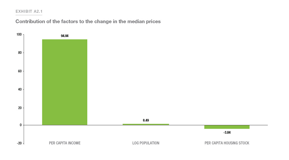
Results of the Oaxaca Blinder Decomposition suggest that these factors (population, per capita income, and per capita housing stock) explain almost 90% of the difference in the median house prices between 2010 and 2019. Median House prices is real median house prices adjusted by CPI less shelter. Incomes is real disposable income.

Of the difference, per capita income explains 94% of the difference between the median house prices in 2010 and 2019. Population explains only around 0.5%, suggesting that it may not have been population that drives house price increases. On the other hand, per capita housing stock has a negative sign, which indicates that housing stock is helping to close the gap between the median house prices: that is, more housing stock is helping reduce the appreciation in house prices.

PREPARED BY THE ECONOMIC & HOUSING RESEARCH GROUP

Sam Khater, Chief Economist
Len Kiefer, Deputy Chief Economist
Venkataramana Yanamandra, Macro Housing Economics Senior
Genaro Villa, Macro Housing Economics Professional