Three Trends That Are Shaping the Future of Housing

I bought my first house in the mid-80s in the suburbs surrounding Kansas City. The area was growing rapidly, and it felt like the neighborhood changed every day between the time I left for work and the time I drove home. Neighbors moved in, neighbors moved out. New schools sprouted up so quickly that our children changed elementary schools twice though we hadn't moved. An upscale grocery appeared a few blocks away where there had been an open field, and the grocery anchored the appearance of other stores and services.

We returned to Kansas City this summer along with some of our former neighbors to attend a wedding—the youngest daughter of the only neighbor to remain in the area. We had some time to kill, so we went to take a look at our old cul-de-sac. We were astonished. We remembered a sun-scorched subdivision with lots of spindly "starter" trees. Now all the houses were shaded by tall, leafy trees. In our time in Kansas City, the rapid changes in the buildings and services focused our attention and dominated our conversations. However, it took over 20 years for us to notice the growth of the trees—a growth that completely changed the ambience of the neighborhood.

A similar phenomenon occurs in housing and mortgage markets. The highest-profile happenings often are the highest-frequency and most transitory, while some of the factors that will determine the future of housing evolve so slowly that we tend to overlook them. For instance, Freddie Mac has published a weekly survey of primary market mortgage rates for over forty years. Each week's survey receives prominent coverage in the press, but each week's survey is promptly forgotten when the subsequent week's numbers are announced.¹

Three long-standing trends—ones that have been building quietly over decades—ultimately will have more influence on housing than the week-to-week oscillations of mortgage rates or any of a host of other short-term indicators of housing activity. These trends will shape the future of housing by permanently shifting both the demand for and supply of housing. These trends don't grab as many headlines, in large part because their impact builds gradually over long spans of time. Nonetheless, no analysis of the future housing market is complete without considering them.

The three trends

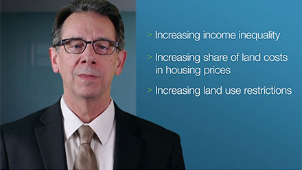
The three trends that are shaping the future of housing are (1) increasing income inequality, (2) an increasing share of land costs in housing prices, and (3) increasing land use restrictions. In this section, we'll describe each of these trends in turn. In the subsequent section, we'll highlight how these trends are likely to shape the U.S. housing market.

Increasing income inequality

The first, and perhaps most important, trend is increasing income inequality. However, we're not talking about the growing gulf between the very-richest Americans and the majority of the population. High-flying executive pay and the lavish lifestyles of the "1 percent" may be eye-catching, but they ultimately have little impact on the $22 trillion American housing market.² The changes in the income distribution that matter to housing are the shifts in the relative fortunes of low-, middle-, and high-skilled workers. These shifts began decades ago, and they continue today.³

A critical feature of the changing job landscape is the polarization of job opportunities. There are three aspects to this polarization.

• First, demand has increased for both high-skilled, high-wage workers and low-skilled, low-wage workers (Exhibit 1); 

  

  

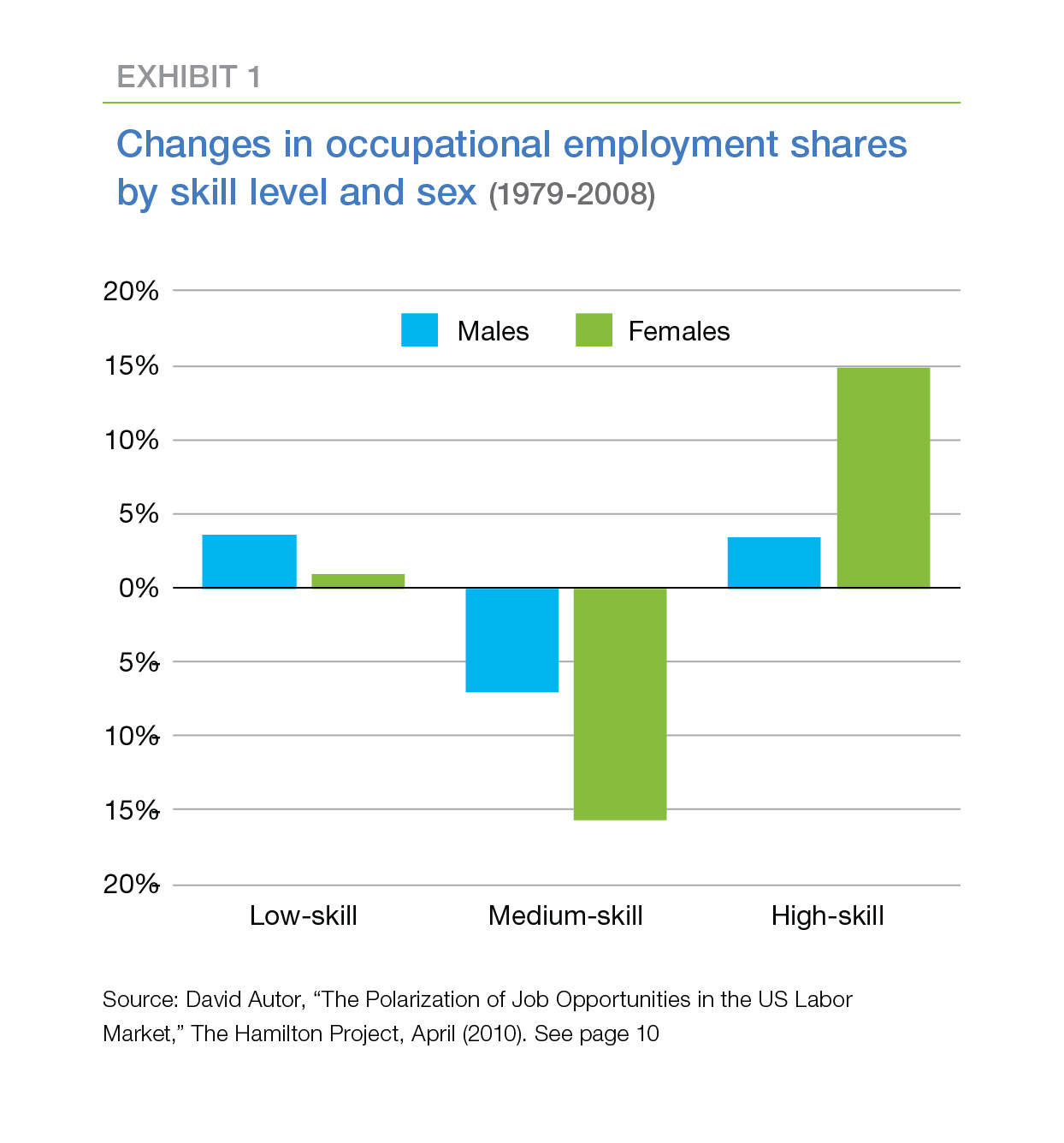
• At the same time, demand for middle-skill jobs has decreased contributing to a "hollowing-out" of the middle class. Technology has eliminated white-collar clerical, blue-collar production and craft, and related jobs. A recent, but typical, example is Walmart's announcement in August that it is laying off 7,000 accounting and invoicing positions.
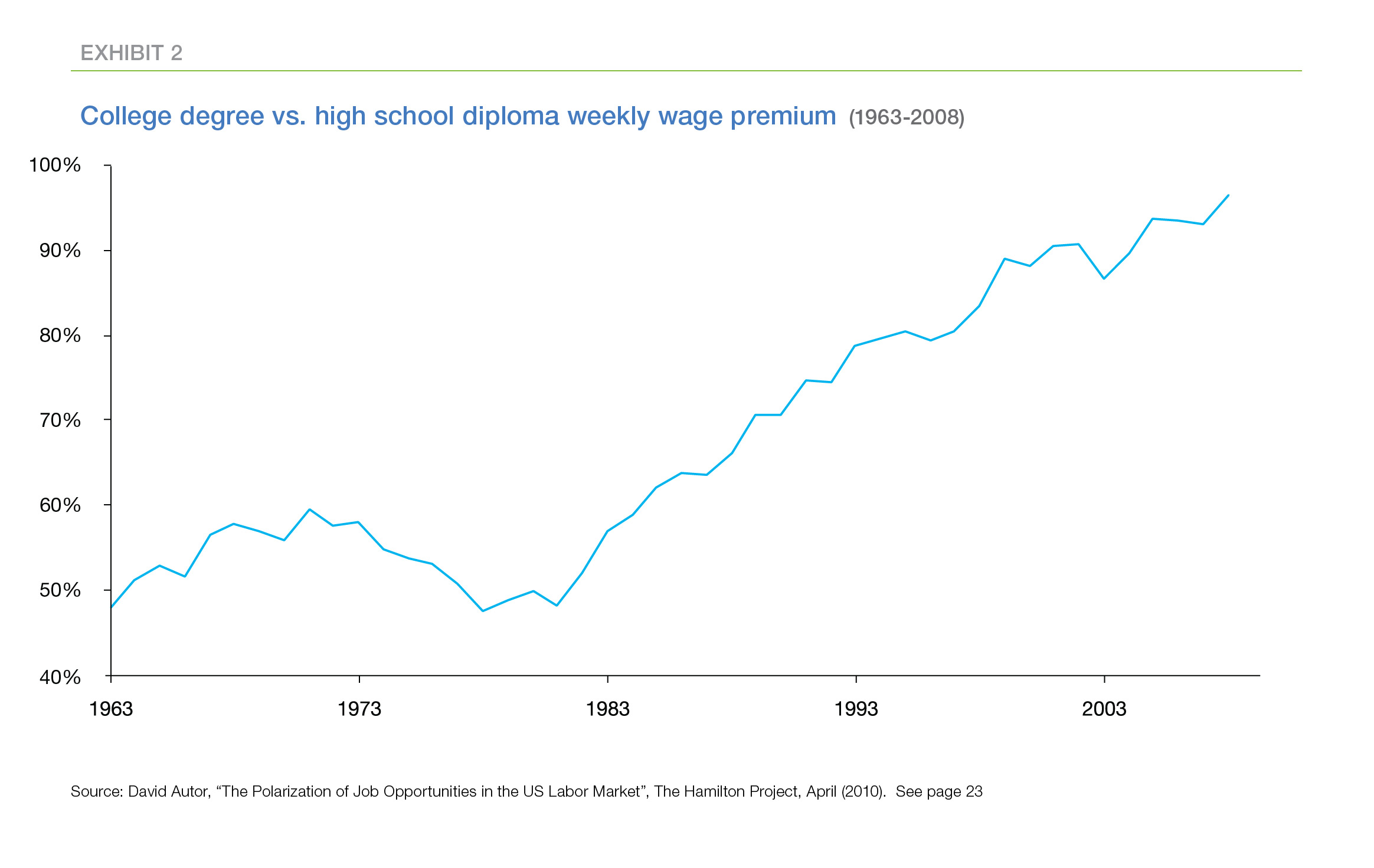
• Finally, the real earnings of college-educated workers have increased while the real earnings of workers without college educations have fallen, magnifying the gap between the earnings of high- and low-skilled workers (Exhibit 2).^4,5 Since the mid-1970s, increasing demand for skilled workers in the U.S. has outpaced U.S. educational attainment. The result has been a significant increase in the inequality of wages. For example, in 1980, workers with four-year college degrees earned 50 percent more per hour than high school graduates. Twenty-eight years later, college graduates earned 95 percent more per hour.⁶

The increasing share of land costs in housing prices

The second trend is the increasing share of land costs in home building. Despite the vast regions of open land in the U.S., buildable land sufficiently close to population and employment centers is scarce. This scarcity is more pronounced in some areas than others. For instance, San Francisco is surrounded on three sides by water, and there is almost no buildable land in the city that hasn't already been developed. Just about the only way to build a new house is first to knock down an old house, and that approach doesn't increase the number of houses.⁷ Other cities are surrounded by undeveloped or lightly developed areas that can absorb new residences. However, even in those cities, new development will be concentrated in areas distant from the center of the city with fewer existing amenities and higher commuting costs to jobs, shopping, health care, etc. Thus, over time, land in prime locations has become relatively scarce and its price has risen.⁸

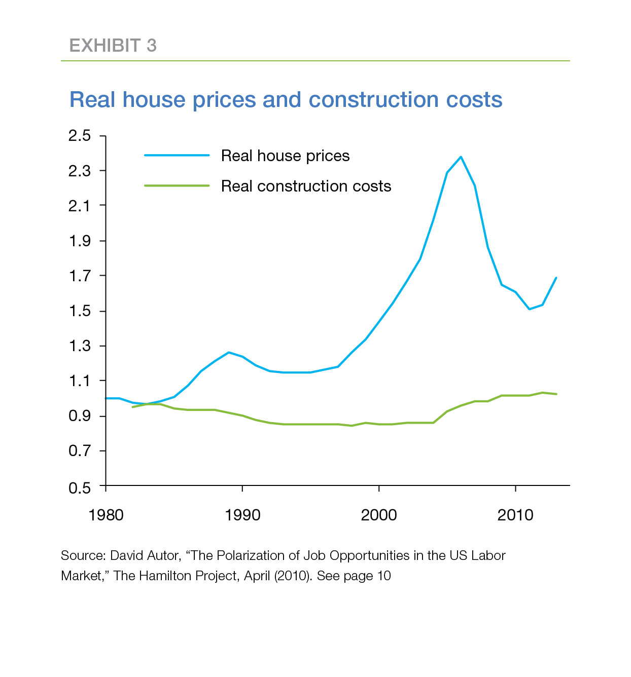
In contrast, real construction costs have risen slowly. As a result, the cost of the land component of a new house has risen faster than construction costs (Exhibit 3). From 1996 to the peak of the mid-2000s housing boom, real house prices more than doubled, however real construction costs increased by only 12 percent. Most of the increase in house prices can be attributed to a sharp rise in land values.⁹ Even today, after real house prices have retreated from their peak and real construction costs have increased another 12 percent, the share of land costs remains much higher than it was in the mid-1990s.

Increasing land use restrictions

A recent paper by Peter Ganong and Daniel Shoag¹⁰ highlights a third, and related, trend. For a century, per capita income grew more rapidly in poorer U.S. states than in richer states. As a result, the income gap between states narrowed. This convergence was fueled by migration; residents of poorer states moved to take advantage of the higher wages available in richer states. This migration held down wage growth in the richer states and boosted it in the poorer states.

Over the past three decades, however, the rate of convergence has slowed. Ganong and Shoag provide evidence that increasingly-strict land use regulations in the richer states are responsible for this slowdown. Regulation has boosted housing costs in richer states, making migration more difficult for low-skilled workers, while leaving it still attractive to high-skilled workers who can earn enough to defray the higher housing costs. The authors estimate the increase in hourly wage inequality from 1980 to 2010 would have been 10 percent smaller if the convergence in state income per capita had maintained its earlier, more rapid pace.¹¹

While the mechanism described by Ganong/Shoag is complex, the authors present a compelling and easily-understood example. Consider two professions—attorney and janitor—two locations—the tri-state area around New York City and the Deep South—and two time periods—1960 and 2010. In both time periods, an attorney's earnings were much higher than a janitor's and the cost of living was much higher in the New York area than in the Deep South. In 1960, the higher wages in New York more than compensated for the higher cost of living for both professions; both the attorney and the janitor were economically better off in New York. However, by 2010, only the attorney was better off in New York. The difference in the cost of living had increased to the point that the janitor was economically better off in the Deep South.¹² As a result, by 2010, workers in low-skill, low-wage professions, such as the janitor, had less of an economic incentive to migrate from a poorer state to a richer state.

Impacts on the housing and mortgage markets

These three trends affect housing and mortgage markets through their influence on both the demand for and the supply of housing. The change in income distribution shifts the demand for housing—both the total demand for homeownership and the demand for different types of housing. The rising share of land costs shifts the supply of housing—houses cost more than before because of the higher cost of the land component of the house. And land use restrictions limit the supply of more-affordable housing in richer states.¹³

Long-term impacts of these trends include:

• A potential boost to the homeownership rate;
• An increase in housing inequality;
• An increase in the volatility of house prices;
• The return of homeownership as an effective means of wealth creation;
• Possible shifts in the FHA/VA, GSE, and private sector shares of the mortgage market.

Let's explore each of these impacts in turn.

Homeownership

The impact on homeownership depends primarily on the way the polarization of jobs shifts the distribution of household incomes. Higher-income households have higher homeownership rates. As a result, the overall impact on the homeownership rate depends on the way that households are pushed out of the middle of the income distribution and toward the extremes. A potential boost to the homeownership rate may occur if future changes in income distribution are similar to changes over the last four decades.¹⁴

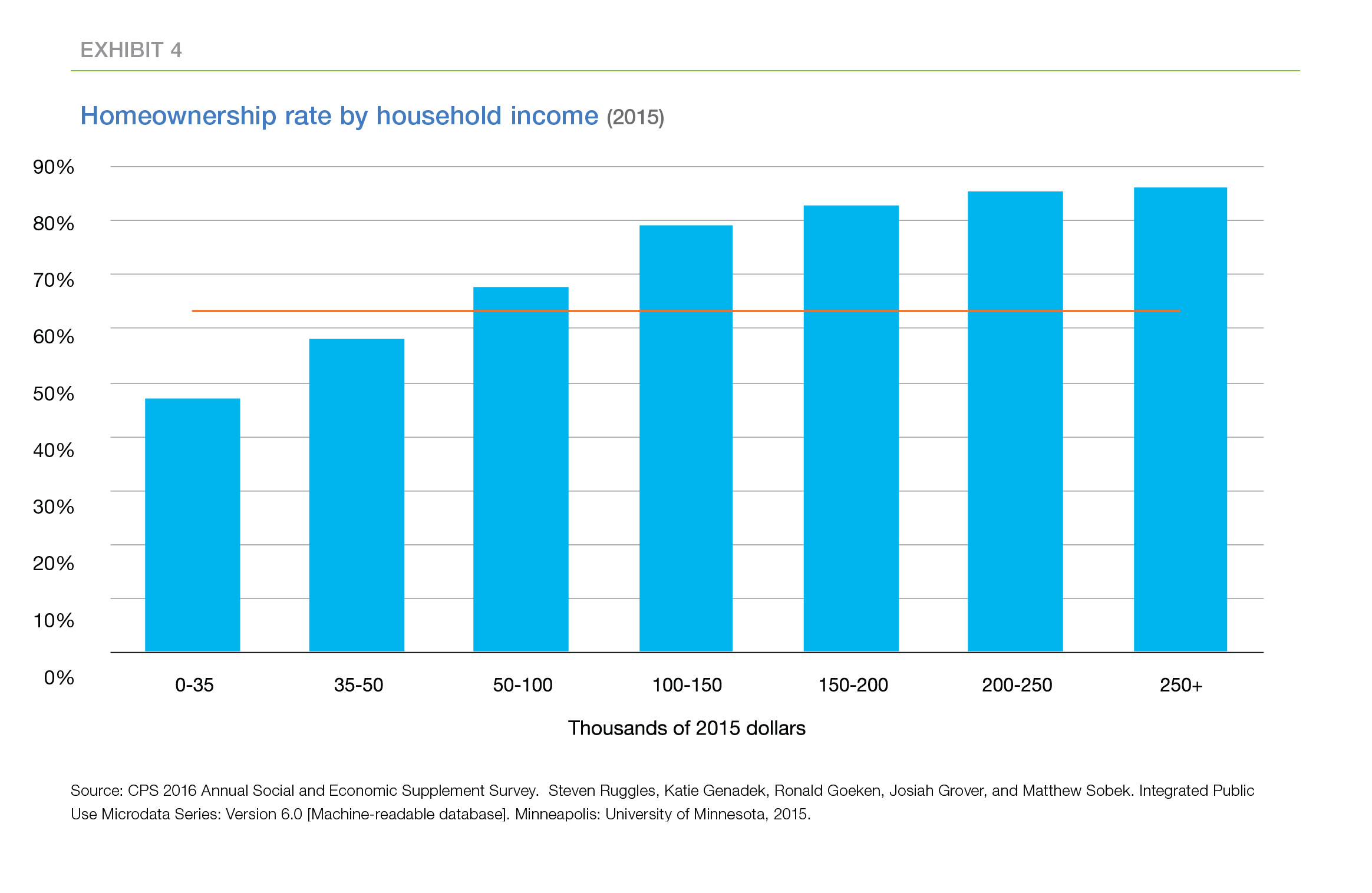
Exhibit 4 displays the relationship between the homeownership rate and household income in 2015. The rate of homeownership increases sharply with household income up to an income of about $150,000, then increases more slowly at higher incomes. The horizontal line at 63.5 percent marks the national homeownership rate in the third quarter of 2016, the most recent reading. Households with annual incomes of $50,000 or less had homeownership rates less than this national average, while households with annual incomes greater than $50,000 had rates greater than the national average.

The trend toward the polarization of jobs (and income) has been in place since the mid-1970s. As a result, the shifts in the income distribution from the 70s to today may be indicative of future shifts in the income distribution. Exhibit 5 compares the income distributions four decades apart, in 1975 and 2015. Exhibit 6 displays the changes in these income shares.

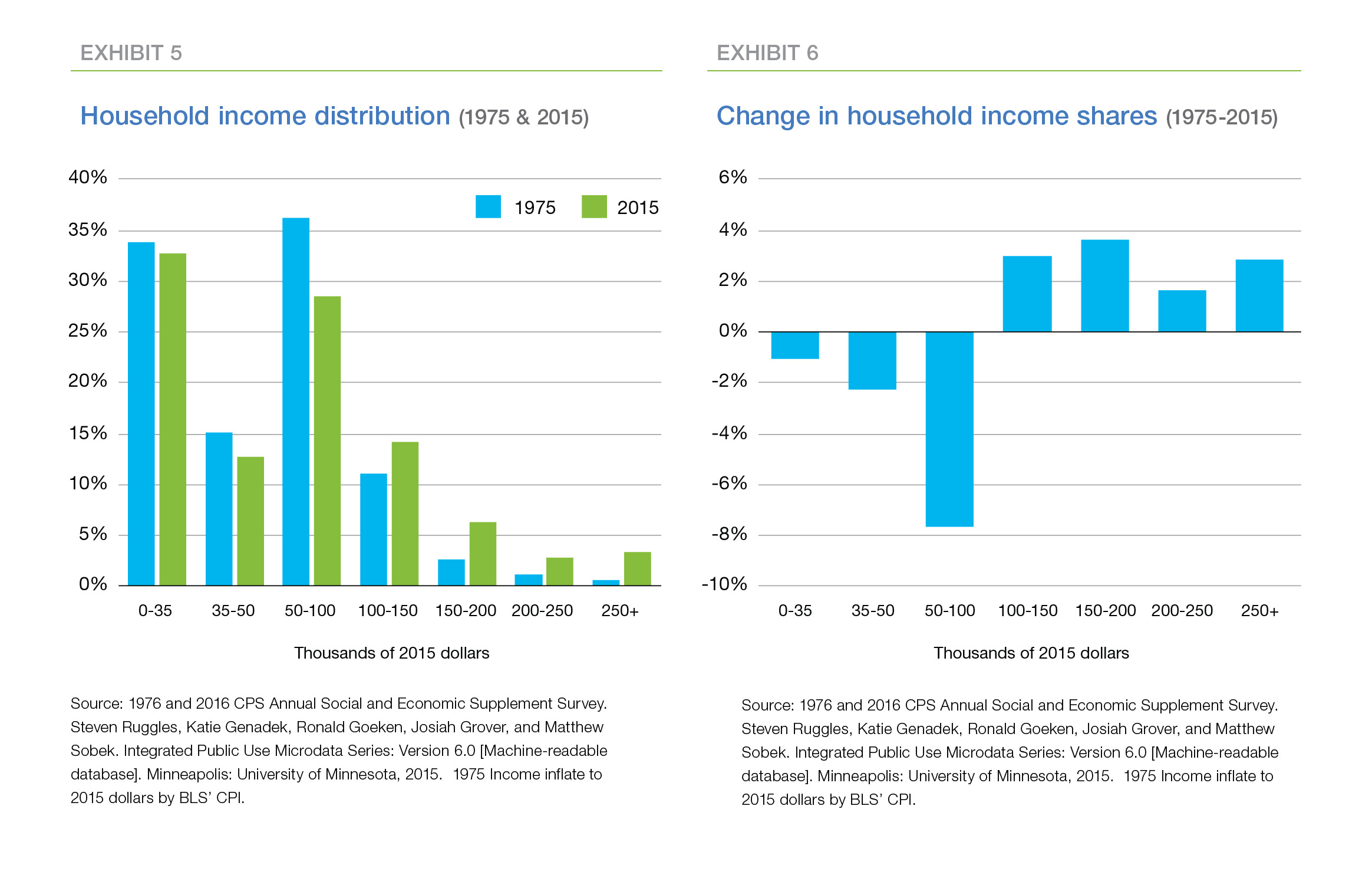
Exhibit 6 is a bit surprising. The trend towards polarization in the job market led us to expect a different pattern than we see in Exhibit 6. The polarization of jobs has increased the demand for both low-skill and high-skill jobs at the expense of middle-skill jobs, and the real wage gap between high-skill and low-skill jobs has increased. Those two facts suggested that the long-run change in the distribution of household income might be U-shaped—more low-income and high-income households and fewer middle class/middle income households. Instead the share of all income categories below $100,000 fell while the share of all higher income categories grew. Thus, as Exhibit 6 shows, there is a much smaller share of middle-income households today than there was 40 years ago and a greater share of upper-income households. However, the share of low-income households has declined slightly rather than grown.

There is no official definition of middle class, but the Pew Research Center suggests classifying households with incomes between two-thirds and two times the median household income as middle class. Using this definition, households with incomes between, roughly, $35,000 and $100,000 qualify as middle class. The share of middle class households fell 10 percentage points between 1975 and 2015, from 51 percent to 41 percent. The share of upper-income households rose 11 percentage points, from 15 percent to 26 percent, while the share of lower-income households fell 1 percentage points, from 34 percent to 33 percent.

This unexpected pattern of change in household income distribution most likely reflects the challenges in tracing changes in the relative wages of low-, middle-, and high-skill workers to changes in the distribution of household income. Consider, for example, Exhibit 7 which displays the household income distributions of these three classes of workers.

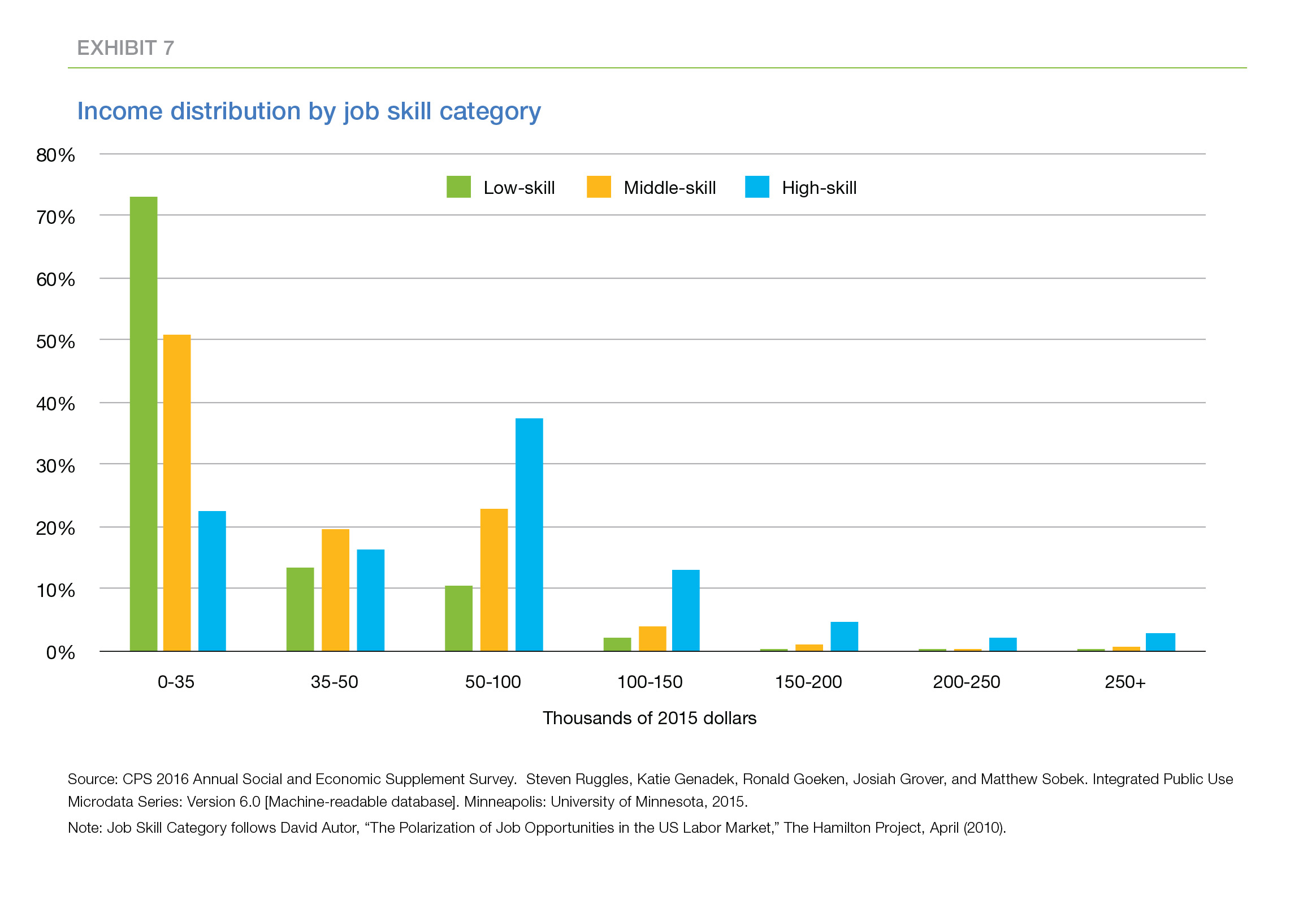
The correspondence between skill levels and household income levels is pretty rough; the growing disparity in the real wages of low-, middle-, and high-skill workers is not reflected in household incomes. For example, the majority of low-skill workers are in low-income households, but 24 percent of low-skill workers are in middle-income households and 3 percent of low-skill workers actually are in high-income households. Similarly, middle- and high-skill workers appear in households at all income levels.

Some of the decline in the share of low-income households over the last 40 years may reflect the improvement in real incomes for all groups over the last 40 years. Within each skill group, the distribution of household incomes has shifted to the right over the past four decades, subtracting population share from the low-income group. In addition, the average number of wage earners per household may have grown over time, increasing household income even where the real wage of each worker in the household failed to increase.

In any event, the income distribution has shifted over the last four decades in a way that favors homeownership. The share of households with lower-than-average homeownership rates has decreased, and the share with higher-than-average rates has increased.

To quantify the potential impact of the continuing trend of polarization on homeownership, assume that the distribution of household incomes changes in the next forty years exactly as it did in the previous forty years. The share in the $35,000-to-$50,000 category falls by two percentage points, the share in the $50,000-to-$100,000 category falls by eight percentage points and so on. Further, assume the relationship between household income and homeownership is unchanged. Under these assumptions, the national homeownership rate will increase three percentage points, from 63 percent in 2016 to 66 percent in 2056.

Housing inequality

Intuitively, the increase in income inequality since the 1970s should be associated with an increase in housing inequality as well, and recent research by David Albouy and Mike Zabek appears to confirm that intuition. (See Exhibit 8, Exhibit 9) Measuring housing inequality is not as simple as comparing the square footage of different houses. There are many aspects of the quality of a housing unit, including the amenities of the neighborhood, such as schools and parks, and distance to economic centers. Albouy and Zabek approach this difficulty by calculating estimates of the consumption value of housing services, that is, an imputed rent.

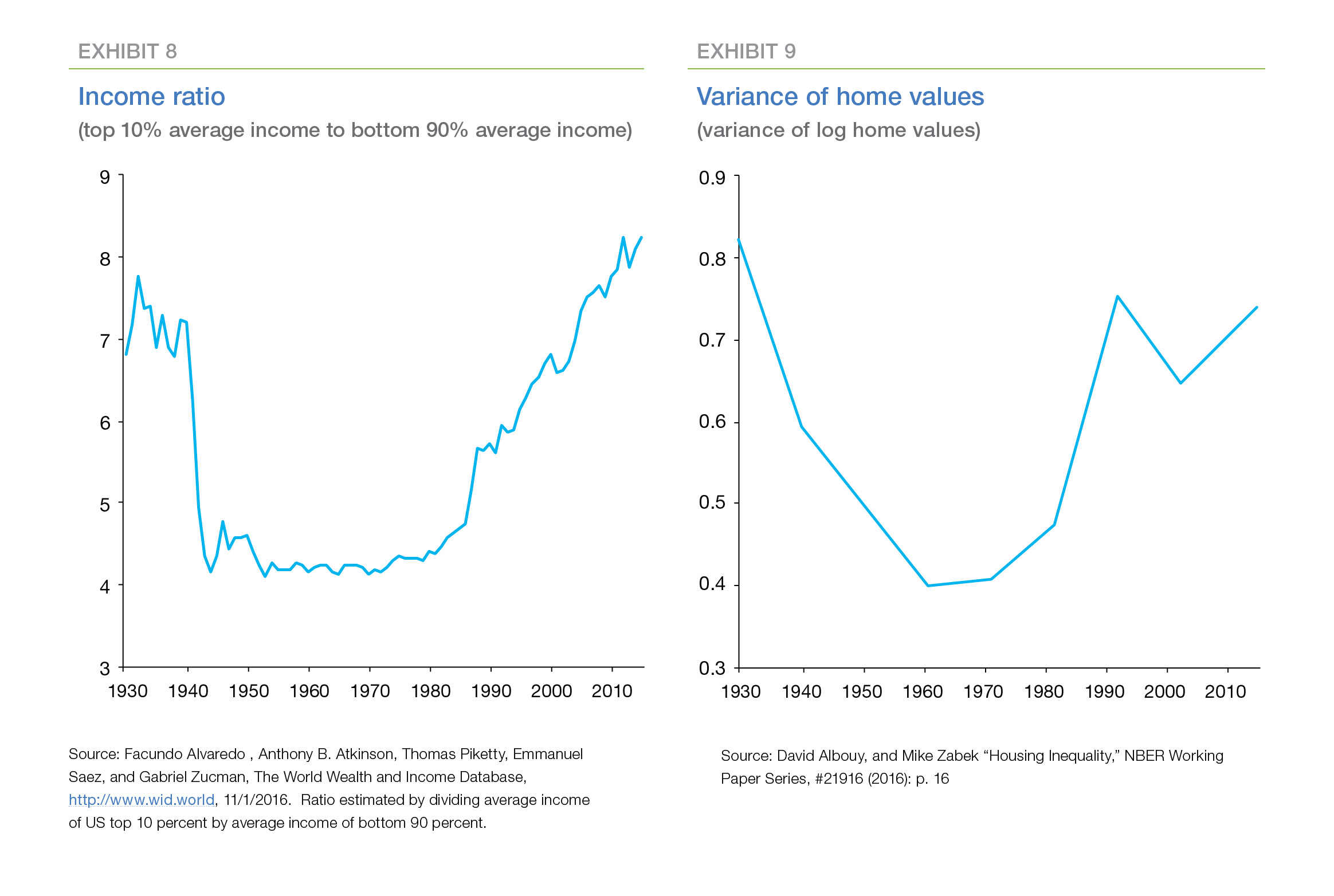
Using these estimates, Albouy and Zabek document a secular increase in housing inequality. They find that housing inequality decreased from 1930 to 1970 as the rate of homeownership increased by almost a third. However, from 1970 to 2012, this trend reversed and housing inequality increased—a pattern that mimics the pattern of income inequality. They also find that inequality is greater within cities than between cities. Since construction costs within cities do not vary much, they conclude that inequality in land values and variations in land use restrictions within cities are responsible for much of the within-city housing inequality.

The volatility of house prices

House prices are more volatile where buildable land is scarce.¹⁵ The rising share of land costs reflects the scarcity of land in areas of high demand and the growth of land use restrictions exacerbates this scarcity by further limiting the use of the available land. As a result, the supply of housing can't readily expand in response to increases in demand for housing.¹⁶

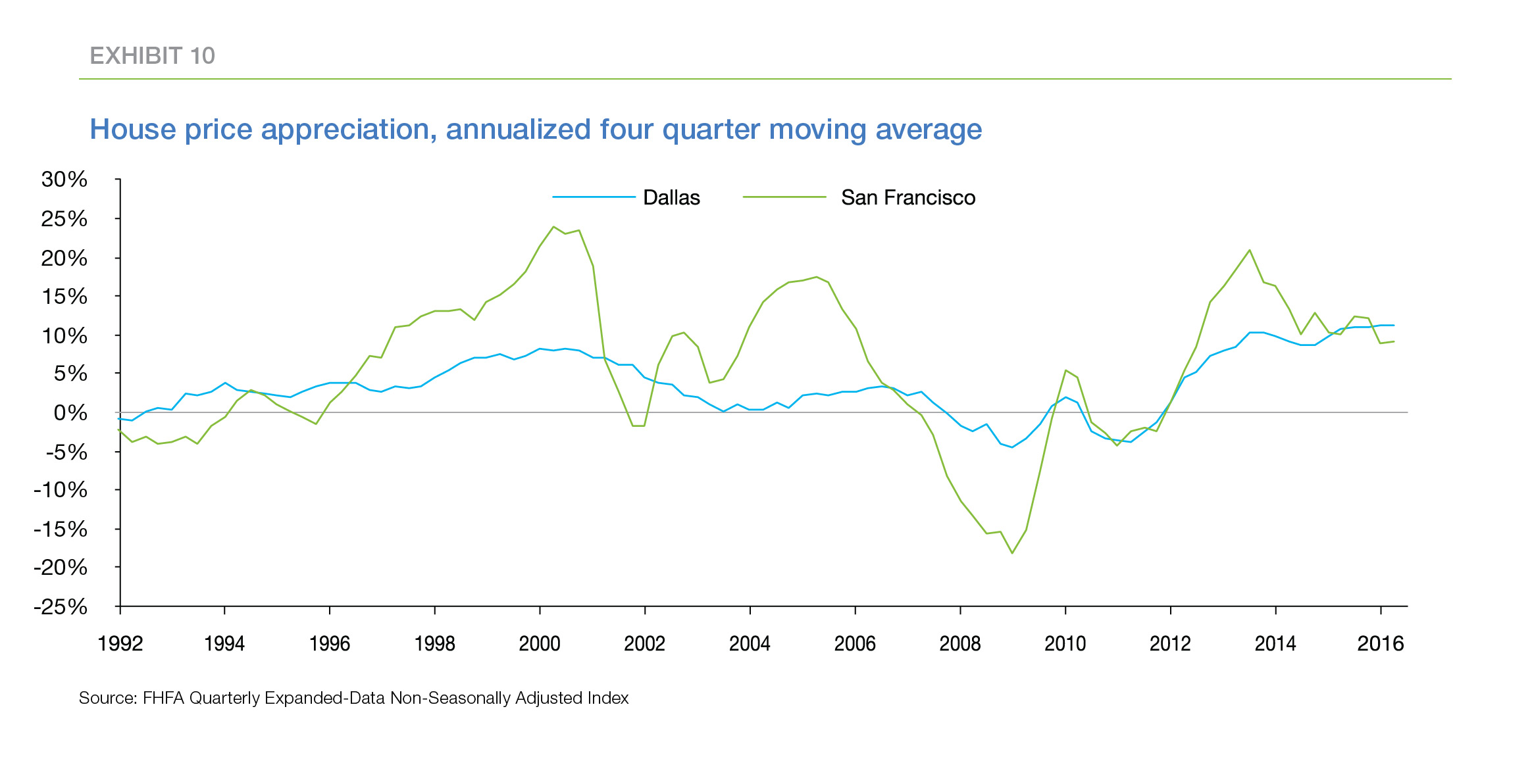
For example, the growth of the tech industry in recent years has attracted more and more people to areas like San Francisco where tech jobs are plentiful. In the absence of sufficient housing to meet the additional demand, potential buyers bid up the price of existing housing. The process works in reverse, as well. The collapse in 2000 of the tech bubble triggered a decline in demand for housing in Silicon Valley, which drove house prices down between five and ten percent.

Exhibit 10 compares house price growth in San Francisco to house price growth in Dallas. Both physical limitations and tight zoning laws make it difficult to increase the supply of housing in San Francisco. In contrast, there is room to spread out in Dallas and zoning laws in Dallas are less restrictive. As a result, house price growth has oscillated more sharply in San Francisco than in Dallas in response to changing economic conditions.¹⁷

Impact on wealth creation through homeownership

The nationwide collapse of house prices in the mid-2000s triggered reconsideration of the assumption that homeownership is an important avenue for wealth creation among working class families. In fact, many families in underserved groups lost both their homes and their hard-earned down payments in the housing crisis, calling the economic benefits of homeownership into question.¹⁸

All three trends suggest that homeownership in richer states and desirable metros will be an effective means of wealth creation. The polarization of jobs is increasing the share of upper income households which in turn is increasing the demand for more-expensive homes. This trend is most pronounced in richer states where land is scarce (and land costs are a larger share of house prices) and land use restrictions limit additions to the supply of housing. The long-term return on housing investment in these locations is likely to be especially high. The returns to investment in housing will likely be smaller in poorer states with more available land and fewer zoning restrictions.

Impacts on mortgage finance

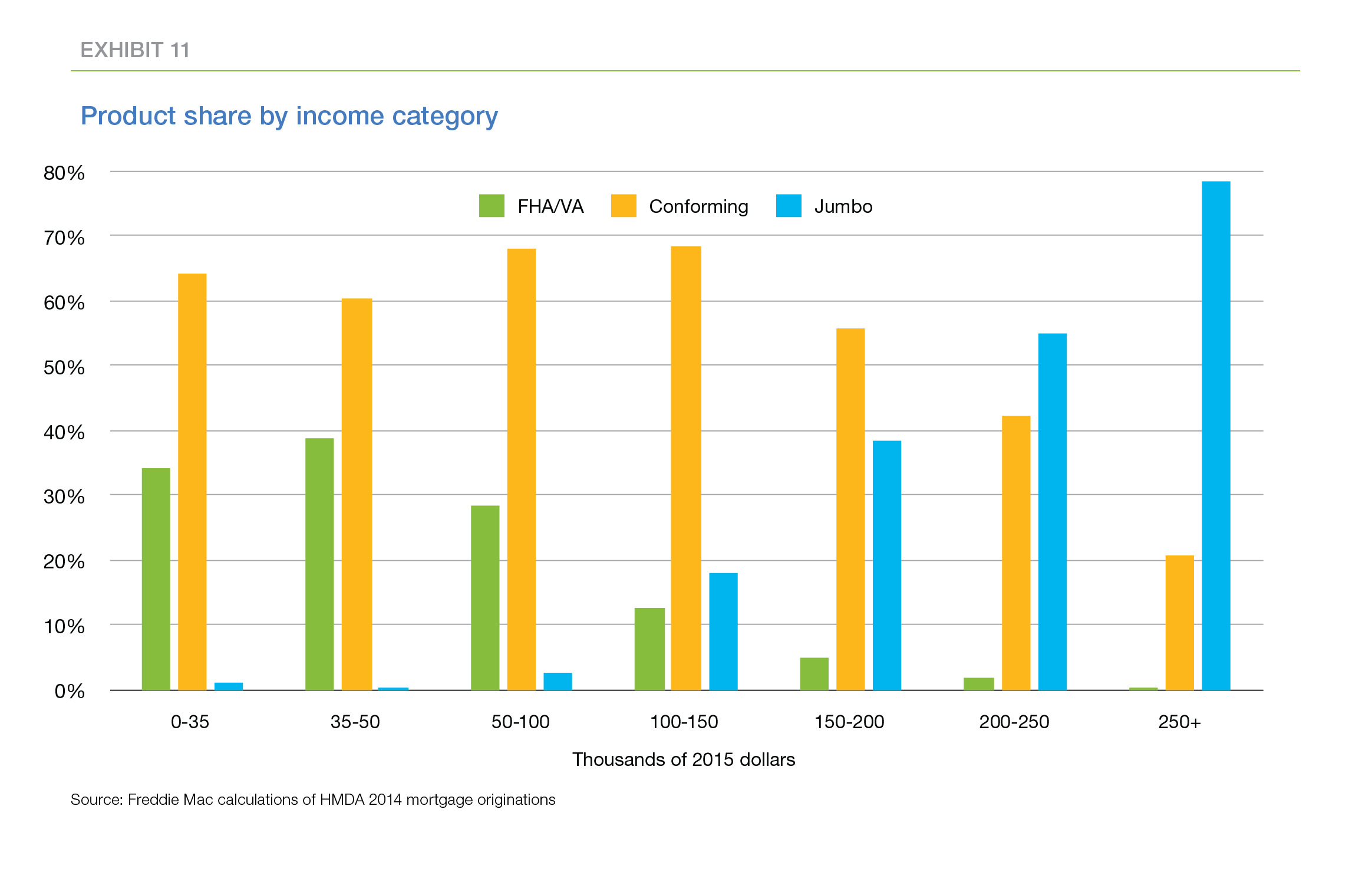
At some risk of oversimplification, the mortgage market can be divided into three somewhat overlapping sectors. The Federal Housing Administration (FHA) and the Veterans Administration (VA) focus on first-time home buyers, lower-income borrowers, and credit-challenged borrowers. The Government-Sponsored Enterprises (GSEs) cover a wider range of mortgage borrowers, providing the bulk of funding to middle-income borrowers while also providing significant funding for other income groups. Banks provide jumbo loans to more affluent borrowers.

Exhibit 11 compares the income distributions of borrowers served by these three sources of mortgage finance. Most of the FHA/VA borrowers are lower-income, although a non-negligible share of middle-income borrowers also take out FHA/VA loans. Virtually all jumbo mortgages are taken out by upper income borrowers. The GSEs provide a significant share of loans to borrowers in all three income classes.¹⁹

The shift in household income distribution discussed above—the reduction in the share of lower- and middle-income households and the increase in the share of upper-income households—is likely to shift the shares of mortgage finance supplied by these three sources over the next few decades. The jumbo share of the market will almost certainly increase as the share of upper-income households in the population grows. The FHA/VA share may plateau or even shrink if the share of lower-income households continues to decline. The impact on the GSEs is difficult to predict, since the GSEs provide mortgage finance across the entire income distribution. And, of course, the influence of future legislative changes in the mortgage finance system could outweigh the impact of the trends in the household income distribution.

Conclusion

Increasing income inequality, the rising share of land costs, and the increase in land use restrictions have developed at a glacial pace compared to the boom and bust of the mid-2000s. As a result, these long-standing trends have escaped the spotlight shone on more recent events. Nonetheless, these three trends will shape the future of housing long after the influence of more recent events plays out.

PREPARED BY THE ECONOMIC & HOUSING RESEARCH GROUP

Sean Becketti, Chief Economist
Brock Lacy, Quantitative Analyst

1 Interestingly, one of the most common requests we receive is for daily, rather than weekly, estimates of mortgage rates.

2 "Table B.101, Owner-occupied real estate including vacant land and mobile homes at market value, series: LM155035015.Q," Federal Reserve Board's Flow of Funds Accounts, September 16, 2016

3 For US trends see: David Autor, "The Polarization of Job Opportunities in the US Labor Market,"The Hamilton Project, April (2010). For International trends see for example : Maarten Goos, and Alan Manning, "Lousy and Lovely Jobs: The Rising Polarization of Work in Britain." Review of Economics and Statistics 89, no. 1 (2007): 118-133.

4 To review these trends see: Lawrence Katz and David Autor,"Changes in the Wage Structure and Earnings Inequality," Handbook of Labor Economics, 3A (1999): 1463-1555, see pages 1476-1480 in particular; David Autor, "The Polarization of Job Opportunities in the US Labor Market,"The Hamilton Project, April (2010), see pages p. 22-23,26-28 for particular examples

5 Jung Hyun Choi and Richard Green provide additional evidence of increasing inequality in incomes across U.S. cities. Their research does not rely directly on the polarization of jobs. However they find that MSAs with a greater share of skilled laborers and a higher share of adults with college degrees tend to have more income inequality.

6 David Autor, "The Polarization of Job Opportunities in the US Labor Market,"The Hamilton Project, April (2010), see page 23.

7 Allowing higher-density development would alleviate some of this scarcity by building multiple residences in a spot that previously held only one. However that approach runs smack dab into the land use restrictions discussed in the next section.

8 Matthew Rognlie, "Deciphering the Fall and Rise in the Net Capital Share: Accumulation or Scarcity?," Brookings Papers on Economic Activity Spring (2015): 1-69. Also Albert Saiz,"The Geographic Determinants of Housing Supply," Quarterly Journal of Economics 125, no. 3 (2010): 1253-1296. For example of more strict zoning and regulatory municipalities see: Joseph Gyourko, Albert Saiz, and Anita Summers, "A New Measure of the Local Regulatory Environment for Housing Markets: The Wharton Residential Land Use Regulatory Index," Urban Studies, 45, no. 3 (2008): 693-729

9 Some of this increase may also reflect the increasing cost of building permits, other fees, and regulation generally. See the next section on land use restrictions.

10 Peter Ganong and Daniel Shoag, "Why Has Regional Income Convergence in the US Declined?,", Hutchins Center Working Paper, #21 (2016): 1-67. For supporting papers see: Paul Beaudry, David A. Green, and Ben Sand “Spatial Equilibrium with Unemployment and Wage Bargaining: Theory and Estimation,” Journal of Urban Economics, 79, (2014): 2-19 Jung Hyun Choi and Richard K. Green “Income Inequality across U.S. Cities,” (2016): 2-39

11 The White House recently issued a report echoing the conclusions of Ganong and Shoag and proposing reductions in local barriers to housing development.

12 The previously-discussed increasing gap in the real wages of high- and low-skill professions also helped tip the balance.

13 In addition, the associated slowdown in regional income convergence may magnify the impact of the growing gap between high-skill and low-skill real wages.

14 Shifts in the age and race/ethnicity distributions also will have an impact on the homeownership rate, and there is reason to believe those shifts may tend to depress the homeownership rate. The boost in the homeownership rate due to changes in the income distribution may be counterbalanced or outweighed by these other factors. See "Why are the Experts Pessimistic About the Future of Homeownership?

15 For simplicity, this section focuses on house prices, but the same argument extends to rents.

16 In economists' terms, supply has become less elastic.

17 In these data, quarterly house price appreciation in San Francisco is more than twice as volatile as in Dallas. Also the average rate of quarterly house price appreciation in San Francisco is 50 percent higher than in Dallas.

18 Robert Shiller "Why Land and Homes Actually Tend to be Disappointing Investments," New York Times, (New York, NY), July 15, 2016, Christopher Herbert, Daniel McCue, and Rocio Sanchez-Moyano "Is Homeownership Still an Effective Means of Building Wealth for Low-Income and Minority Households? (Was it Ever?)," Joint Center For Housing Studies, Harvard University, September (2013)

19 Not all conforming loans are sold to the GSEs, but these shares provide a reasonable guide to the GSE share of each income category.